Ch 13 — Sequential Data
Markov models, hidden Markov models, the forward–backward and Viterbi algorithms, linear dynamical systems.
So far observations have been i.i.d. Real data are often sequences: speech frames, sentences, time series, sensor readings. The challenge is modeling temporal dependence without making the parameter count blow up.
PRML Ch 13 covers the classical hierarchy: Markov models for observations, hidden Markov models for discrete latent state, and linear dynamical systems for continuous latent state. All three share an inference machinery (forward–backward) and learning algorithm (EM, where the M-step is a Markov-chain MLE).
Prerequisites
- Graphical models (Ch 8) — these models are all chain-structured DAGs.
- EM (Ch 9) — Baum–Welch is EM specialized to HMMs.
- Multivariate Gaussians (Ch 2) — for LDSs.
13.1 Markov Models
Order-\(M\) Markov assumption: \(p(x_t \mid x_1, \ldots, x_{t-1}) = p(x_t \mid x_{t-M}, \ldots, x_{t-1})\). The case \(M = 1\) is the first-order Markov model:
\[p(x_1, \ldots, x_T) = p(x_1) \prod_{t=2}^{T} p(x_t \mid x_{t-1}). \tag{13.1}\]For categorical observations with \(K\) states, this is parameterized by an initial distribution \(\boldsymbol{\pi}\) and a transition matrix \(\mathbf{A}\) with \(A_{jk} = p(x_t = k \mid x_{t-1} = j)\). MLE for both is just counting (with smoothing for unseen transitions).
Higher-order Markov needs \(K^M\) parameters — exponential growth. The latent-variable models below are the smarter alternative.
13.2 Hidden Markov Models
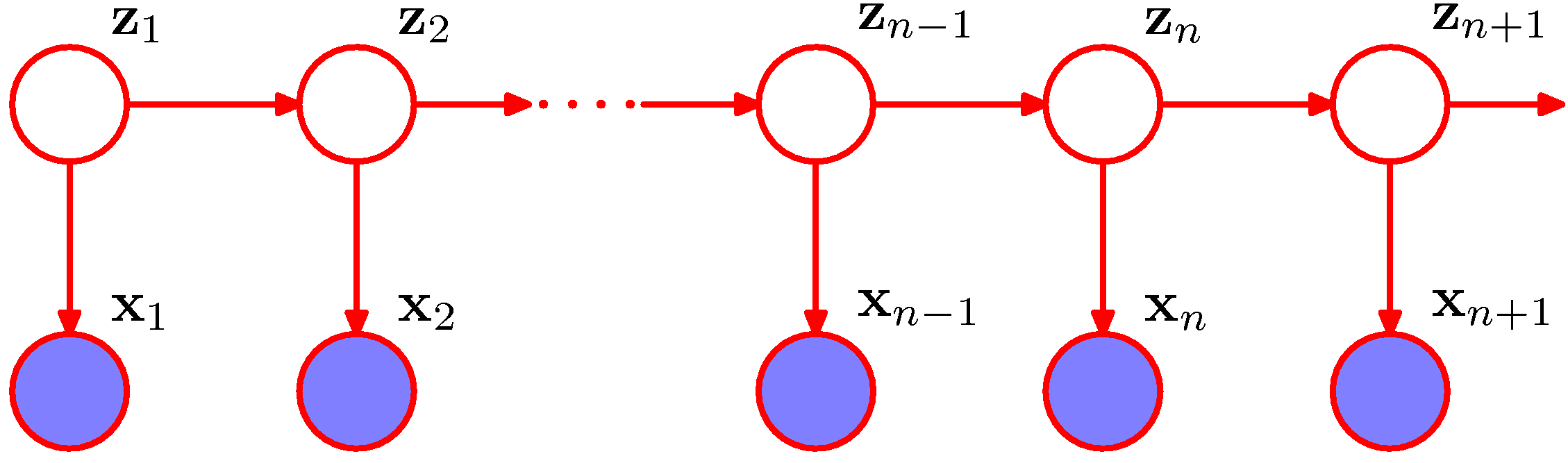
Observations \(\mathbf{x}_1, \ldots, \mathbf{x}_T\) generated from a hidden discrete state sequence \(\mathbf{z}_1, \ldots, \mathbf{z}_T\):
\[p(\mathbf{X}, \mathbf{Z}) = p(\mathbf{z}_1) \prod_{t=2}^{T} p(\mathbf{z}_t \mid \mathbf{z}_{t-1}) \prod_{t=1}^{T} p(\mathbf{x}_t \mid \mathbf{z}_t). \tag{13.2}\]Three sets of parameters:
- Initial distribution \(\pi_k = p(z_{1k} = 1)\).
- Transition matrix \(A_{jk} = p(z_{tk} = 1 \mid z_{t-1, j} = 1)\).
- Emission distributions \(p(\mathbf{x}_t \mid \mathbf{z}_t)\) — Gaussians for continuous \(\mathbf{x}\), categorical for discrete.
Three classical computations:
| Problem | Algorithm | Cost |
|---|---|---|
| Likelihood \(p(\mathbf{X})\) | Forward | \(O(T K^2)\) |
| Posterior marginals \(p(z_t \mid \mathbf{X})\) | Forward–backward | \(O(T K^2)\) |
| Most likely state path | Viterbi | \(O(T K^2)\) |
| MLE of parameters | Baum–Welch (EM) | \(O(T K^2)\) per iteration |
Forward and backward recursions
Define \(\alpha_t(k) = p(\mathbf{x}_1, \ldots, \mathbf{x}_t,\, z_{tk} = 1)\) — the joint probability of observations up to time \(t\) and ending in state \(k\). It satisfies
\[\alpha_t(k) = p(\mathbf{x}_t \mid z_{tk} = 1) \sum_{j=1}^{K} A_{jk}\, \alpha_{t-1}(j),\]with \(\alpha_1(k) = \pi_k\, p(\mathbf{x}_1 \mid z_{1k} = 1)\). The total likelihood is \(p(\mathbf{X}) = \sum_k \alpha_T(k)\).
The backward recursion \(\beta_t(k) = p(\mathbf{x}_{t+1}, \ldots, \mathbf{x}_T \mid z_{tk} = 1)\) similarly satisfies \(\beta_t(k) = \sum_j A_{kj}\, p(\mathbf{x}_{t+1} \mid z_{t+1, j} = 1)\, \beta_{t+1}(j)\). Together they give
\[p(z_{tk} = 1 \mid \mathbf{X}) \propto \alpha_t(k)\, \beta_t(k).\]Viterbi
Replace the sum in the forward recursion with a max:
\[\delta_t(k) = p(\mathbf{x}_t \mid z_{tk} = 1) \max_j A_{jk}\, \delta_{t-1}(j),\]tracking back-pointers as you go. Reading them out at the end yields the maximum-a-posteriori state sequence.
Baum–Welch (EM for HMMs)
E-step: forward–backward to get \(p(z_t \mid \mathbf{X})\) and pairwise \(p(z_t, z_{t+1} \mid \mathbf{X})\). M-step: re-estimate \(\boldsymbol{\pi}\), \(\mathbf{A}\), and the emission parameters using these expected counts. Provably non-decreasing in log-likelihood; converges to a local optimum.
Where HMMs shine
- Speech recognition (the canonical historical application — phones as latent states).
- POS tagging and named-entity recognition (linear-chain CRFs, HMMs’ discriminative cousins).
- Bioinformatics — gene-finding, sequence alignment.
- Activity recognition from sensor data.
Modern deep-learning replacements (RNNs, transformers) often outperform HMMs in raw accuracy but lose the interpretable state structure and the calibrated probabilities.
13.3 Linear Dynamical Systems
The same chain structure as an HMM, but with continuous Gaussian latent states and Gaussian transitions/emissions:
\[\mathbf{z}_t = \mathbf{A}\mathbf{z}_{t-1} + \mathbf{w}_t, \qquad \mathbf{x}_t = \mathbf{C}\mathbf{z}_t + \mathbf{v}_t,\]with \(\mathbf{w}_t \sim \mathcal{N}(\mathbf{0}, \boldsymbol{\Gamma})\), \(\mathbf{v}_t \sim \mathcal{N}(\mathbf{0}, \boldsymbol{\Sigma})\). Because everything is Gaussian, all conditionals stay Gaussian, and the forward–backward equations close in a finite-dimensional state.
Kalman filter and smoother
- Filter (forward pass) — compute \(p(\mathbf{z}_t \mid \mathbf{x}_{1:t})\) sequentially. Two steps per time: a predict (propagate uncertainty through the dynamics) and an update (incorporate the new observation).
- Smoother (backward pass) — compute \(p(\mathbf{z}_t \mid \mathbf{x}_{1:T})\) using all observations. Adds Rauch–Tung–Striebel backward recursions.
The Kalman filter is everywhere: aerospace navigation (its original application), tracking, sensor fusion, robot localization.
Learning
EM applied to LDSs gives closed-form M-steps (linear regressions for \(\mathbf{A}, \mathbf{C}\); covariance averages for \(\boldsymbol{\Gamma}, \boldsymbol{\Sigma}\)). For nonlinear dynamics, fall back to the extended Kalman filter (linearize around the current estimate) or unscented Kalman filter (deterministic sigma points), or move to particle filters for fully nonlinear / non-Gaussian models.
13.4 Beyond PRML: RNNs and Beyond
PRML predates the deep-learning era. The line of descent:
- HMM / LDS (parametric, Gaussian / categorical states).
- RNN / LSTM / GRU (continuous high-dimensional latent state computed by a neural network; trained by BPTT). No closed-form inference, but capacity scales easily.
- Transformers (no recurrence; attention captures long-range dependencies; trained on huge corpora). Now dominate sequence modeling.
The classical models still matter: small-data regimes, interpretable state structure, and as inspiration for modern hybrid models.
Takeaways
- Markov assumption lets you trade exponential parameter growth (in raw history) for a chain-structured factorization.
- HMMs add a discrete latent state; the forward–backward and Viterbi algorithms make exact inference feasible at \(O(T K^2)\).
- LDSs are the Gaussian analog; the Kalman filter is the canonical example.
- EM (Baum–Welch / LDS-EM) is the standard learning algorithm; modern practice often replaces both with RNNs or transformers, trading interpretability for capacity.
Forward to Ch 14 — Combining Models.
Figures from Bishop, Pattern Recognition and Machine Learning (Springer, 2006), © Springer / C. M. Bishop. Reproduced for educational use.