Ch 14 — Combining Models
Bayesian model averaging, committees, boosting, decision trees, conditional mixtures of experts.
A single model is rarely the best you can do. Combining several models — averaging them, voting, stacking, gating — almost always wins on real-world benchmarks. This chapter walks through the main combination strategies and explains why they help.
Prerequisites
- Bias–variance intuition (Ch 3) — most ensemble methods reduce variance, bias, or both.
- Decision theory (Ch 1) — expected loss arguments justify averaging.
- Linear / logistic regression (Chs 3–4) — base learners for boosting.
14.1 Bayesian Model Averaging vs Mixtures
Two ideas often confused:
- Bayesian model averaging. You have a single true model \(h\); you don’t know which member of a family it is. Predictions average over the posterior over models:
As \(N \to \infty\), the posterior concentrates on a single model and BMA is no different from picking that one.
- Mixture model. Different parts of the data are generated by different components. Even with infinite data, the components remain — they describe different mechanisms.
These look similar but say very different things. Ensemble methods below mostly correspond to mixture-style combinations.
14.2 Committees and Bagging
Train \(K\) different models and average their predictions. The simplest case: bootstrap the training set \(K\) times, train a model on each, average — bagging (bootstrap aggregating).
Why does it help? For squared loss with a single regression target,
\[\mathbb{E}\\!\left[\\!\left( \tfrac{1}{K}\sum_k y_k - h \right)^{2} \right] \;\leq\; \frac{1}{K} \sum_k \mathbb{E}\bigl[(y_k - h)^{2}\bigr],\]with equality iff the errors of the individual models are perfectly correlated. Bagging reduces variance without increasing bias — a free lunch when models are noisy and roughly uncorrelated.
Random Forests
Bagging applied to decision trees, with an extra trick: at each split, only a random subset of features is considered. This decorrelates trees further, since a strong feature can’t dominate every tree’s first split. Random forests are frighteningly competitive baselines in tabular data — sometimes the best model, almost always in the top three.
14.3 Boosting
A different ensemble idea: train models sequentially, each focusing on examples the previous models got wrong. AdaBoost (Freund and Schapire) is the prototype:
- Start with uniform weights \(w_n^{(1)} = 1/N\) on training examples.
- For \(m = 1, \ldots, M\):
- Train a weak classifier \(y_m(\mathbf{x})\) minimizing weighted error \(\epsilon_m = \sum_n w_n^{(m)} \mathbb{I}[y_m(\mathbf{x}_n) \neq t_n]\).
- Compute \(\alpha_m = \tfrac{1}{2}\ln \tfrac{1 - \epsilon_m}{\epsilon_m}\).
- Update weights: \(w_n^{(m+1)} \propto w_n^{(m)} \exp(-\alpha_m t_n y_m(\mathbf{x}_n))\), normalizing.
- Predict by sign of \(\sum_m \alpha_m y_m(\mathbf{x})\).
Why boosting works
AdaBoost is forward stagewise additive modeling with the exponential loss \(\exp(-t y)\). At each step, you find the weak learner and weight that most reduce the loss. The exponential loss penalizes mistakes much more harshly than logistic loss, which is why boosting is so aggressive at fitting hard examples — and why it can overfit if pushed too far.
Gradient boosting
Replace the exponential loss with any differentiable loss. At each iteration, fit a weak learner to the negative gradient of the loss (the “pseudo-residuals”). This recovers AdaBoost for exp-loss, gradient boosted regression for squared loss, gradient boosted logistic for log-loss.
XGBoost / LightGBM / CatBoost are modern, scalable gradient-boosting implementations. They’re the standard winners on tabular Kaggle competitions and the gold standard for many production tabular ML tasks.
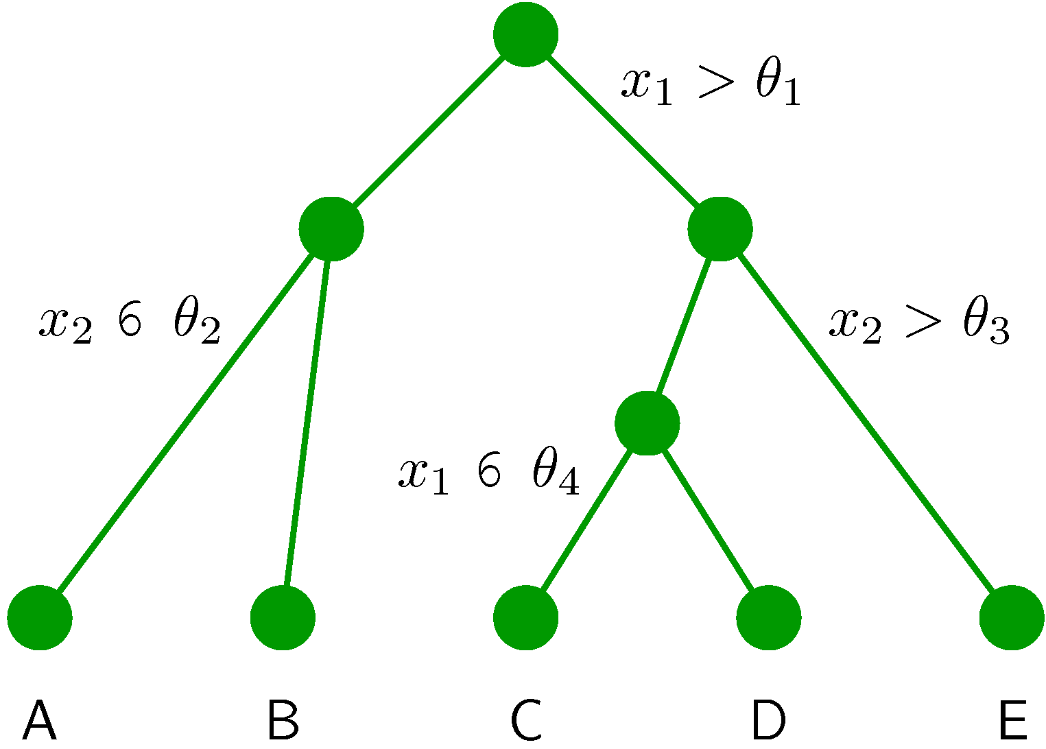
14.4 Decision Trees
A non-linear model that combines well with everything above. Recursively partition the input space: at each node, pick a feature and threshold, route examples left/right. Leaves predict a constant (regression) or a class distribution (classification).
Splitting criteria
- Regression: minimize within-leaf variance.
- Classification: minimize Gini impurity \(1 - \sum_k p_k^{2}\) or entropy \(-\sum_k p_k \log p_k\).
Pros and cons
- + Handles mixed feature types; no scaling needed.
- + Interpretable for small trees.
- + Captures nonlinear interactions automatically.
- − High variance; tiny data perturbations can produce very different trees.
- − Prone to overfit; needs depth control or pruning.
The high-variance flaw is what makes trees ideal building blocks for ensembles — random forests and gradient boosting both lean on tree variance to drive ensemble diversity.
14.5 Conditional Mixtures (Mixture of Experts)
A gating network decides which expert handles each input:
\[p(t \mid \mathbf{x}) = \sum_{k=1}^{K} g_k(\mathbf{x})\, p_k(t \mid \mathbf{x}), \qquad \sum_k g_k(\mathbf{x}) = 1.\]The gates \(g_k(\mathbf{x})\) are typically softmax outputs of a small network. The experts \(p_k\) are arbitrary base models. EM trains both jointly: E-step assigns soft responsibilities; M-step retrains the experts and gates.
Recent revival in deep learning: sparse mixture of experts (Switch Transformer, GLaM) routes each token to only \(k\) of \(N\) experts, dramatically increasing parameter count without proportional compute. Same conceptual structure, modern implementation.
14.6 Stacking
Train base learners on the training data; train a meta-learner to combine their predictions on a held-out fold. Generalizes weighted averaging — the meta-learner can find non-linear combinations.
In practice: blend ~5–10 strong base models (random forest, gradient boosting, logistic regression, k-NN, SVM) via a ridge or logistic meta-learner. Reliable winning recipe in tabular ML competitions.
14.7 Choosing an Ensemble
- Tabular data, lots of structure: gradient boosting (LightGBM, XGBoost) — usually best.
- Tabular, want quick baseline: random forest — fast and competitive.
- Want interpretable features and decisions: single decision tree, or extract feature importances from a forest.
- Image / text: ensemble of neural networks — train several with different seeds, average predictions (“deep ensembles”). Calibrated, robust uncertainty.
- Small data with diverse base models: stacking.
Takeaways
- Bagging averages over bootstrap-trained models — variance reduction, no bias change.
- Boosting trains sequentially, focusing on hard examples — bias reduction at the cost of overfitting risk.
- Random forests combine bagging with feature subsampling; gradient boosting generalizes AdaBoost to any differentiable loss.
- Mixture of experts routes inputs to specialized sub-models; the modern sparse variant scales to enormous parameter counts.
- Stacking combines diverse base learners through a meta-learner — essentially always the recipe for a Kaggle-tier tabular pipeline.
That closes out the PRML curriculum. From here the natural next reads are:
- Bishop & Bishop (2024), Deep Learning: Foundations and Concepts — modern continuation of this material.
- Murphy, Probabilistic Machine Learning (2 vols, 2022 / 2023) — encyclopedic update of PRML.
- Goodfellow, Bengio & Courville, Deep Learning (2016) — focused on neural network methodology.
Figures from Bishop, Pattern Recognition and Machine Learning (Springer, 2006), © Springer / C. M. Bishop. Reproduced for educational use.