Ch 12 — Continuous Latent Variables (PCA)
Principal component analysis, probabilistic PCA, factor analysis, kernel PCA, ICA, autoencoders.
Many high-dimensional datasets live near a low-dimensional manifold. Principal component analysis (PCA) is the simplest and most-used tool for finding that manifold — a linear one. This chapter starts with classical PCA, gives it a probabilistic interpretation that lets EM and Bayesian methods apply, then generalizes to nonlinear (kernel PCA, autoencoders) and statistically richer (ICA) variants.
Prerequisites
- Linear algebra: eigendecomposition, SVD, projections.
- Multivariate Gaussians (Ch 2) — probabilistic PCA is a Gaussian latent-variable model.
- EM (Ch 9) — useful for the missing-data and large-D cases.
12.1 Classical PCA
Two equivalent definitions:
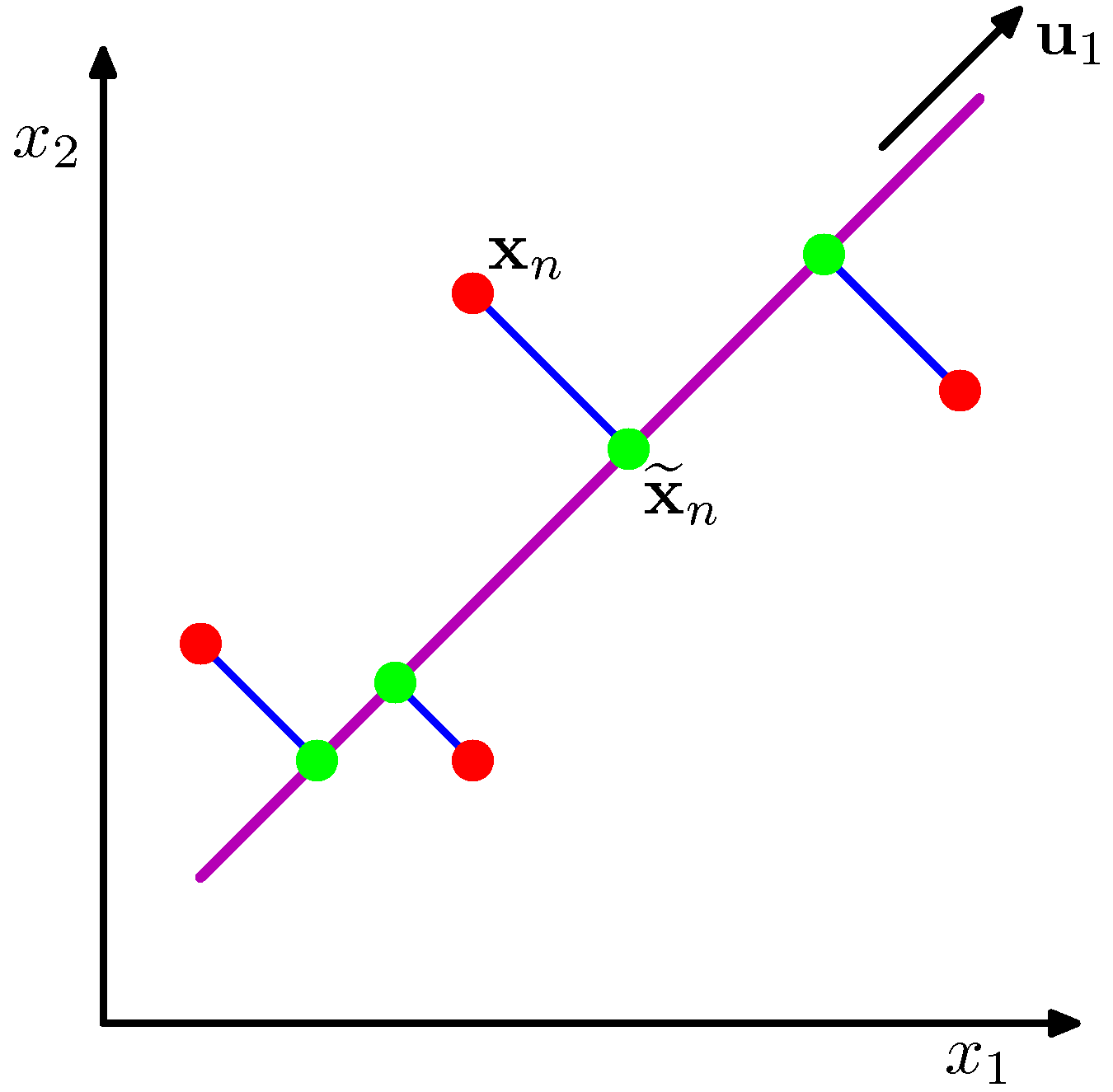
- Maximum-variance projection. Find unit vectors \(\mathbf{u}_1, \ldots, \mathbf{u}_M\) such that the projected data \(\mathbf{u}_j^{\top}\mathbf{x}\) has maximum variance, subject to \(\mathbf{u}_j^{\top}\mathbf{u}_k = \delta_{jk}\).
- Minimum-reconstruction-error projection. Find an \(M\)-dim subspace minimizing \(\sum_n \|\mathbf{x}_n - \widehat{\mathbf{x}}_n\|^2\) where \(\widehat{\mathbf{x}}_n\) is the projection of \(\mathbf{x}_n\) onto the subspace.
The two definitions yield the same answer: the \(\mathbf{u}_j\) are the eigenvectors of the data covariance \(\mathbf{S} = \frac{1}{N}\sum_n (\mathbf{x}_n - \bar{\mathbf{x}})(\mathbf{x}_n - \bar{\mathbf{x}})^{\top}\) with the \(M\) largest eigenvalues. The principal components \(z_{nj} = \mathbf{u}_j^{\top}(\mathbf{x}_n - \bar{\mathbf{x}})\) are the new coordinates.
Computation: SVD
In practice you compute PCA via the SVD of the centered data matrix \(\mathbf{X}_c = \mathbf{U} \boldsymbol{\Sigma} \mathbf{V}^{\top}\). The columns of \(\mathbf{V}\) are the principal directions; the singular values are \(\sqrt{N \lambda_i}\). The SVD is numerically stabler than computing \(\mathbf{S}\) explicitly.
Choosing \(M\)
Plot the eigenvalue spectrum and look for an “elbow.” For a more principled answer, the probabilistic-PCA framework below allows Bayesian model selection.
12.2 Probabilistic PCA
A latent-variable model: \(\mathbf{z} \sim \mathcal{N}(\mathbf{0}, \mathbf{I}_M)\), \(\mathbf{x} = \mathbf{W}\mathbf{z} + \boldsymbol{\mu} + \boldsymbol{\epsilon}\) with \(\boldsymbol{\epsilon} \sim \mathcal{N}(\mathbf{0}, \sigma^{2}\mathbf{I}_D)\). Marginalizing out \(\mathbf{z}\):
\[p(\mathbf{x}) = \mathcal{N}(\mathbf{x} \mid \boldsymbol{\mu},\; \mathbf{W}\mathbf{W}^{\top} + \sigma^{2} \mathbf{I}). \tag{12.1}\]Maximum likelihood for \((\mathbf{W}, \sigma^{2}, \boldsymbol{\mu})\) has a closed-form solution — the columns of \(\mathbf{W}\) span the principal subspace, and \(\sigma^{2}\) is the average of the discarded eigenvalues. Classical PCA is recovered as \(\sigma^{2} \to 0\).
Why the probabilistic view is worth the trouble
- EM can fit PCA without ever forming the \(D \times D\) covariance matrix — useful when \(D\) is large.
- Missing data falls out naturally: marginalize over the missing components in the E-step.
- Bayesian PCA with a prior on \(\mathbf{W}\) gives automatic relevance determination of the latent dimension — the model prunes columns it doesn’t need.
- Mixtures of probabilistic PCAs model data as drawn from one of several local linear subspaces. Useful when one global subspace is too rigid.
Factor Analysis
The same model with diagonal but non-isotropic noise covariance: \(\boldsymbol{\epsilon} \sim \mathcal{N}(\mathbf{0}, \boldsymbol{\Psi})\) with \(\boldsymbol{\Psi}\) diagonal. Less restrictive than PPCA; common in psychometrics and finance. Loses the closed-form ML solution but EM still works.
12.3 Kernel PCA
PCA finds the principal axes of the covariance matrix \(\frac{1}{N}\sum_n (\mathbf{x}_n - \bar{\mathbf{x}})(\mathbf{x}_n - \bar{\mathbf{x}})^{\top}\). What if you first map to a feature space \(\boldsymbol{\phi}(\mathbf{x})\) and PCA there?
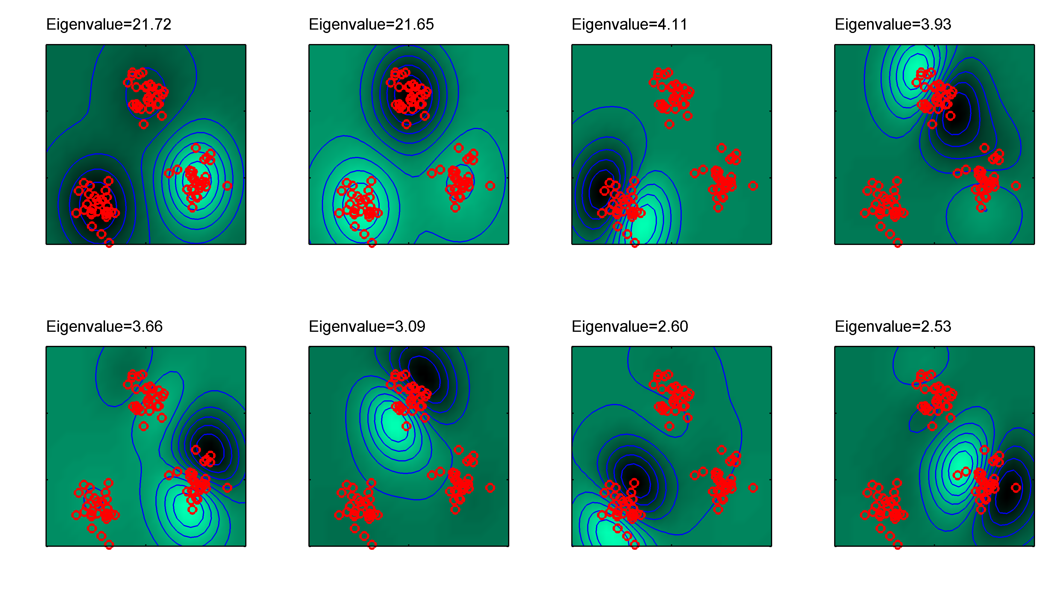
Working out the dual, you find the principal coordinates \(z_{nj}\) are computed from the Gram matrix \(K_{nm} = k(\mathbf{x}_n, \mathbf{x}_m)\) (with appropriate centering): they’re proportional to the eigenvectors of \(\mathbf{K}\). Same kernel trick as Ch 6 — implicit nonlinear features, explicit only through pairwise evaluations.
Kernel PCA produces nonlinear principal components — useful for visualizing data on a curved manifold, or as a preprocessing step for downstream classifiers.
12.4 Independent Component Analysis (ICA)
Suppose your observations are linear mixtures of statistically independent, non-Gaussian sources: \(\mathbf{x} = \mathbf{A}\mathbf{s}\) with \(\mathbf{s}\) independent components. ICA recovers \(\mathbf{s}\) by finding a linear unmixing that maximizes statistical independence (or, equivalently, non-Gaussianity by central-limit-theorem reasoning).
The classical use case is cocktail-party / blind source separation: separate \(n\) speakers recorded by \(n\) microphones. Doesn’t assume Gaussian sources — that’s the whole point.
PCA decorrelates; ICA fully decouples. They’re complementary.
12.5 Modern: Autoencoders
Take a neural network with a bottleneck, train to reconstruct its input: \(\mathbf{x} \to \mathbf{z} \to \widehat{\mathbf{x}}\), minimizing \(\|\mathbf{x} - \widehat{\mathbf{x}}\|^{2}\). The bottleneck \(\mathbf{z}\) plays the role of the latent code.
- Linear autoencoder (no nonlinearities) recovers PCA up to a rotation.
- Nonlinear autoencoder generalizes to nonlinear manifolds — same role kernel PCA plays, but learnable end-to-end.
- Denoising / variational variants regularize the latent space (force robustness to input noise; force \(q(\mathbf{z}\mid\mathbf{x})\) to match a prior).
Variational autoencoders (VAEs) are the modern probabilistic version — Ch 10’s ELBO + the reparameterization trick.
Takeaways
- PCA = top eigenvectors of the data covariance = top right singular vectors of the centered data matrix.
- Probabilistic PCA is a Gaussian latent-variable model; closed-form MLE recovers PCA, and the formulation enables EM, missing-data handling, and Bayesian model selection.
- Kernel PCA runs PCA in an implicit feature space — nonlinear principal components.
- ICA finds independent (non-Gaussian) components; PCA only decorrelates.
- Autoencoders are the modern, learnable, possibly probabilistic counterpart — and the bridge to deep generative models.
Forward to Ch 13 — Sequential Data (HMMs, LDS).
Figures from Bishop, Pattern Recognition and Machine Learning (Springer, 2006), © Springer / C. M. Bishop. Reproduced for educational use.