Ch 11 — Sampling Methods
Rejection and importance sampling, Metropolis–Hastings, Gibbs sampling, slice sampling, Hamiltonian Monte Carlo.
When we can’t write down a closed-form posterior, can’t approximate it well variationally, or simply need samples for a downstream task, stochastic approximation comes in. The objects of interest are usually expectations under a complicated distribution: \(\mathbb{E}_p[f(\mathbf{z})] = \int f(\mathbf{z}) p(\mathbf{z})\, \mathrm{d}\mathbf{z}\). If we can draw samples \(\mathbf{z}^{(t)} \sim p\), the sample average \(\frac{1}{T}\sum f(\mathbf{z}^{(t)})\) converges to the integral. The rest of this chapter is about how to sample.
Prerequisites
- Probability density basics (Ch 2) — knowing what proposals, ratios, and acceptance probabilities mean.
- Markov chains — stationary distributions, detailed balance.
- Some patience — sampling diagnostics.
11.1 Basic Sampling
Inverse-CDF and rejection sampling
If \(p\) is 1-D and you can compute its CDF \(F\), draw \(u \sim \mathrm{Uniform}(0,1)\) and return \(F^{-1}(u)\). Exact but limited: most distributions of interest don’t have invertible CDFs.
Rejection sampling. Pick an envelope \(q(\mathbf{z})\) and constant \(M\) with \(M q(\mathbf{z}) \geq \widetilde{p}(\mathbf{z})\) for all \(\mathbf{z}\) (where \(\widetilde{p}\) is the unnormalized target). Draw \(\mathbf{z} \sim q\), \(u \sim \mathrm{Uniform}(0, M q(\mathbf{z}))\); accept if \(u \leq \widetilde{p}(\mathbf{z})\). Acceptance rate is \(Z/M\). In high dimensions \(M\) is forced to grow exponentially → rejection sampling fails as \(D\) grows.
Importance sampling
Don’t sample from \(p\); sample from \(q\) and reweight:
\[\mathbb{E}_p[f] = \int f(\mathbf{z})\, \frac{p(\mathbf{z})}{q(\mathbf{z})} q(\mathbf{z})\, \mathrm{d}\mathbf{z} \approx \frac{1}{T} \sum_{t=1}^{T} f(\mathbf{z}^{(t)})\, \frac{p(\mathbf{z}^{(t)})}{q(\mathbf{z}^{(t)})}.\]The variance is finite iff \(q\) has heavier tails than \(p\). Catastrophic failure mode: a single sample with huge weight dominates the estimate. Practical rule: monitor the effective sample size \(\mathrm{ESS} = \big(\sum w_t\big)^{2} / \sum w_t^{2}\); restart if too low.
11.2 Markov Chain Monte Carlo
For high dimensions, ditch the global proposal and walk a Markov chain whose stationary distribution is the target.
Metropolis–Hastings
At state \(\mathbf{z}\), propose \(\mathbf{z}^{\star} \sim q(\mathbf{z}^{\star} \mid \mathbf{z})\); accept with probability
\[A(\mathbf{z}^{\star}, \mathbf{z}) = \min\\!\left(1, \frac{\widetilde{p}(\mathbf{z}^{\star})\, q(\mathbf{z} \mid \mathbf{z}^{\star})}{\widetilde{p}(\mathbf{z})\, q(\mathbf{z}^{\star} \mid \mathbf{z})}\right). \tag{11.1}\]This satisfies detailed balance, so the chain’s stationary distribution is \(p\). Run long enough and discard a burn-in; the rest are dependent samples from \(p\).
Tuning the proposal scale matters enormously. Too small: random walk, slow mixing. Too large: most proposals rejected, slow mixing. Aim for ~25 % acceptance in 1-D, dropping to ~23 % asymptotically (the optimal value for random-walk Metropolis as \(D \to \infty\)).
Gibbs sampling
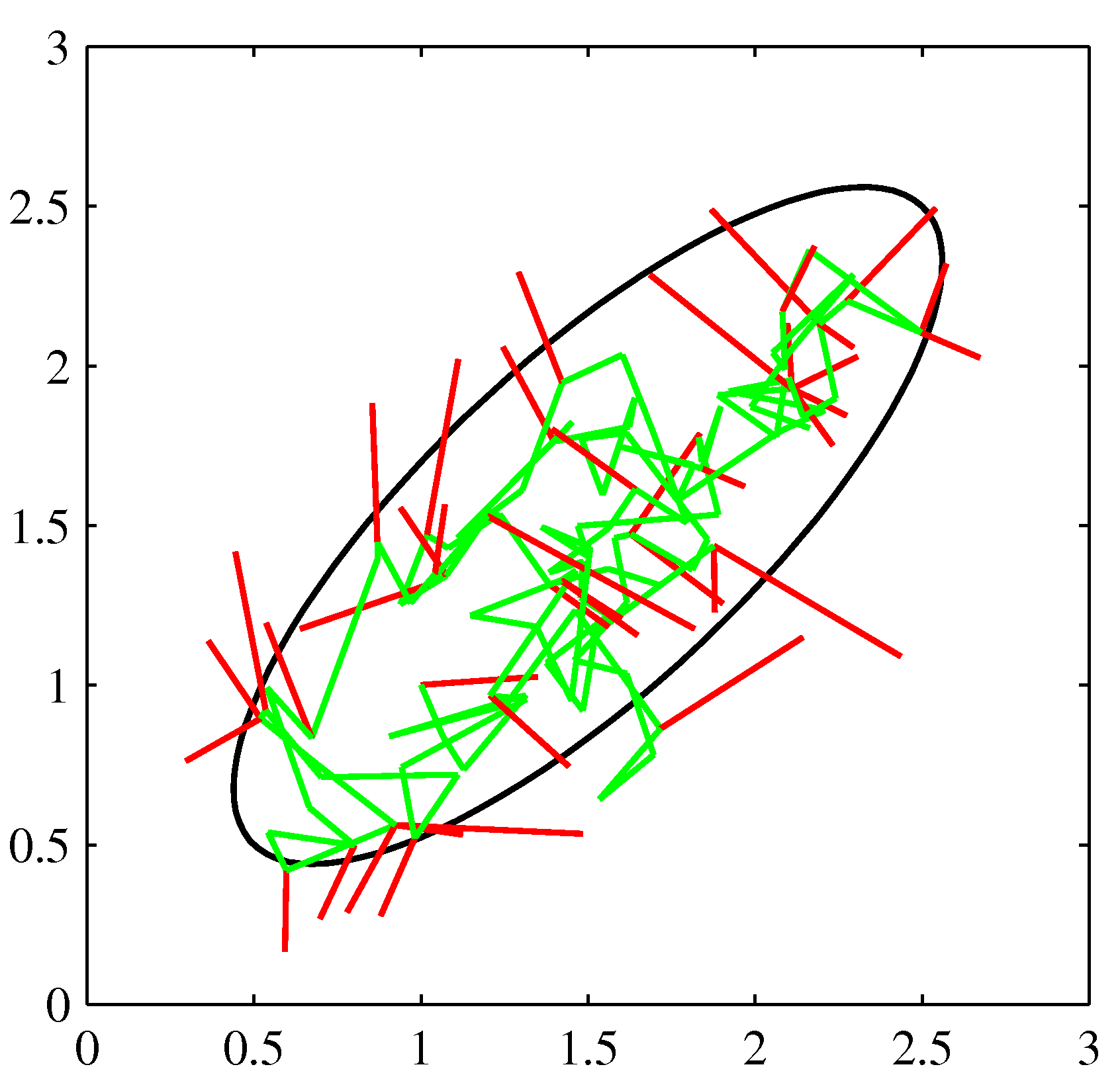
Special case of Metropolis–Hastings where the proposal is the conditional posterior of one variable given all others:
\[\mathbf{z}_i^{(t+1)} \sim p(\mathbf{z}_i \mid \mathbf{z}_{\setminus i}^{(t)}). \tag{11.2}\]Acceptance probability is always 1 (a feature, not a coincidence — derive it). Gibbs is the natural sampler for graphical models where conditional posteriors are simple closed forms (Beta-Bernoulli, Dirichlet-multinomial, conjugate Gaussians).
Limitation: variables that are highly correlated under \(p\) get updated one at a time, producing slow mixing along correlation directions. Standard fixes: block-Gibbs (sample groups jointly), reparameterization, or HMC.
Slice sampling
Auxiliary-variable trick: introduce an auxiliary \(u\) such that \(p(\mathbf{z}, u) \propto \mathbf{1}[0 \leq u \leq p(\mathbf{z})]\). Alternate sampling \(u \mid \mathbf{z}\) (uniform on \([0, p(\mathbf{z})]\)) and \(\mathbf{z} \mid u\) (uniform on the slice \(\lbrace \mathbf{z} : p(\mathbf{z}) \geq u\rbrace\)). The marginal over \(\mathbf{z}\) is \(p\). Adapts step sizes automatically; minimal tuning.
Hamiltonian Monte Carlo
The killer app of modern MCMC. Treat \(\mathbf{z}\) as a “position” and introduce momentum \(\mathbf{r} \sim \mathcal{N}(\mathbf{0}, \mathbf{M})\). The joint distribution \(\propto \exp(-H(\mathbf{z}, \mathbf{r}))\), where \(H = -\ln p(\mathbf{z}) + \tfrac{1}{2}\mathbf{r}^{\top}\mathbf{M}^{-1}\mathbf{r}\), is the Boltzmann distribution at temperature 1. Integrate Hamilton’s equations for some time \(T\) using a leapfrog scheme; accept the endpoint via a Metropolis correction (compensating for discretization error).
The trajectory follows the gradient of the log-target, so HMC moves long distances in correlated regions where random-walk Metropolis would crawl. The cost is an extra gradient evaluation per leapfrog step. Most heavy-duty Bayesian inference today (Stan, PyMC, NumPyro) is HMC under the hood, with the No-U-Turn Sampler (NUTS) auto-tuning the trajectory length.
11.3 Convergence Diagnostics
MCMC samples are dependent and start from arbitrary states — you need to verify the chain has reached its stationary distribution before trusting estimates.
- Burn-in. Discard the first ~10–50 % of samples.
- Trace plots. Eyeball each variable’s chain — should look like white noise around a stable mean.
- Autocorrelation function. Should decay; effective sample size \(N_{\mathrm{eff}}\) is \(N / (1 + 2 \sum \rho_k)\) where \(\rho_k\) is the autocorrelation at lag \(k\).
- Multi-chain \(\widehat{R}\) (Gelman–Rubin). Run several chains from different starts; compare within-chain to across-chain variance. \(\widehat{R} < 1.01\) is the typical “converged” threshold.
If \(\widehat{R}\) is high or \(N_{\mathrm{eff}}\) is tiny, don’t trust the estimates. Reparameterize, use HMC, or add tempering.
11.4 When to Use Sampling vs Variational
| Sampling | Variational | |
|---|---|---|
| Exact in the limit | Yes | No (always approximate) |
| Wall-clock time | Hours to days for hard models | Minutes to hours |
| Fits with mini-batches | Awkward (SGLD, etc.) | Naturally |
| Reliable on multimodal posteriors | Hard but doable (parallel tempering) | Mean-field collapses to one mode |
| Predictive uncertainty | High-fidelity samples | Often under-estimated |
| Rule of thumb | Models with thousands of parameters | Models with millions/billions |
For a small Bayesian regression: NUTS is the right answer. For a Bayesian neural network with millions of weights: variational, dropout, or ensembles.
Takeaways
- Rejection and importance sampling are conceptually simple but break down in high dimensions.
- MCMC trades exact independence for a Markov chain that has \(p\) as its stationary distribution. Metropolis–Hastings is the master template; Gibbs is the conjugate-friendly special case.
- HMC / NUTS is the modern default for continuous, smooth posteriors — moves long distances along gradients, vastly outperforming random-walk Metropolis in correlated targets.
- Diagnostics matter. \(\widehat{R}\), \(N_{\mathrm{eff}}\), and trace plots are non-negotiable.
Forward to Ch 12 — Continuous Latent Variables (PCA).
Figures from Bishop, Pattern Recognition and Machine Learning (Springer, 2006), © Springer / C. M. Bishop. Reproduced for educational use.