Ch 2 — Probability Distributions

← Intro to ML

Density estimation — the problem of modeling $p(\mathbf{x})$ from a finite dataset — is fundamentally underconstrained: infinitely many distributions are consistent with any finite sample. To make progress we choose a parametric family and pick the best member of that family for our data. This chapter walks through the canonical families: Bernoulli for binary outcomes, multinomial for categorical, Gaussian for continuous, and the unifying exponential family that encompasses all of them.

For each, we cover three things:

The distribution itself — formula, mean, variance, when to use it.
Maximum likelihood — the recipe-style point estimate.
A conjugate prior — turning that point estimate into a Bayesian posterior with closed-form updates.

Prerequisites for this chapter

Probability: sum/product rules, joint vs marginal vs conditional, expectation. (Reviewed in Ch 1.)
Calculus: differentiating a log-likelihood and setting it to zero. Lagrange multipliers for constrained optimization (for the multinomial MLE).
Linear algebra: matrix inverses, determinants, quadratic forms — needed once we hit multivariate Gaussians.

2.1 Binary Variables

The Bernoulli distribution

Let $x \in \lbrace 0, 1\rbrace$ with $p(x = 1) = \mu$. Then $p(x = 0) = 1 - \mu$, and we can compactly write

\[\operatorname{Bern}(x \mid \mu) = \mu^{x}(1 - \mu)^{1 - x}. \tag{2.1}\]

Sanity check on the exponent trick:

If $x = 1$: the second term becomes $(1 - \mu)^{0} = 1$, leaving $\mu$. ✓
If $x = 0$: the first term becomes $\mu^{0} = 1$, leaving $1 - \mu$. ✓

Mean and variance follow directly: $\mathbb{E}[x] = \mu$ and $\operatorname{var}[x] = \mu(1 - \mu)$ — the variance peaks at $\mu = 1/2$ (a fair coin is the most uncertain binary outcome).

Maximum likelihood for $\mu$

Suppose we observe $\mathcal{D} = \lbrace x_1, \ldots, x_N\rbrace$ — the outcomes of $N$ independent flips. Treating the flips as i.i.d., the likelihood is

\[p(\mathcal{D} \mid \mu) = \prod_{n=1}^{N} \mu^{x_n}(1 - \mu)^{1 - x_n}.\]

Take the natural logarithm to convert the product into a sum (much easier to differentiate):

\[\ln p(\mathcal{D} \mid \mu) = \sum_{n=1}^{N} \lbrace x_n \ln \mu + (1 - x_n) \ln(1 - \mu) \rbrace.\]

Differentiate with respect to $\mu$ and set to zero:

\[\frac{\partial}{\partial \mu} \ln p(\mathcal{D} \mid \mu) = \sum_{n=1}^{N} \left( \frac{x_n}{\mu} - \frac{1 - x_n}{1 - \mu} \right) = 0.\]

Multiply through by $\mu(1 - \mu)$ and rearrange:

\[\sum_{n=1}^{N} \lbrace x_n (1 - \mu) - (1 - x_n) \mu \rbrace = \sum_{n=1}^{N} (x_n - \mu) = 0,\]

\[\boxed{\,\mu_{\mathrm{ML}} = \frac{1}{N} \sum_{n=1}^{N} x_n = \frac{m}{N}\,} \tag{2.2}\]

where $m$ is the number of heads (1’s) observed. The MLE is just the sample frequency — exactly what intuition suggests.

Caveat — overfitting in the small-$N$ limit. If you flip a coin $N=3$ times and see all heads, $\mu_{\mathrm{ML}} = 1$, predicting that every future flip will be heads with certainty. Bayesian methods fix this (next subsection).

The binomial distribution

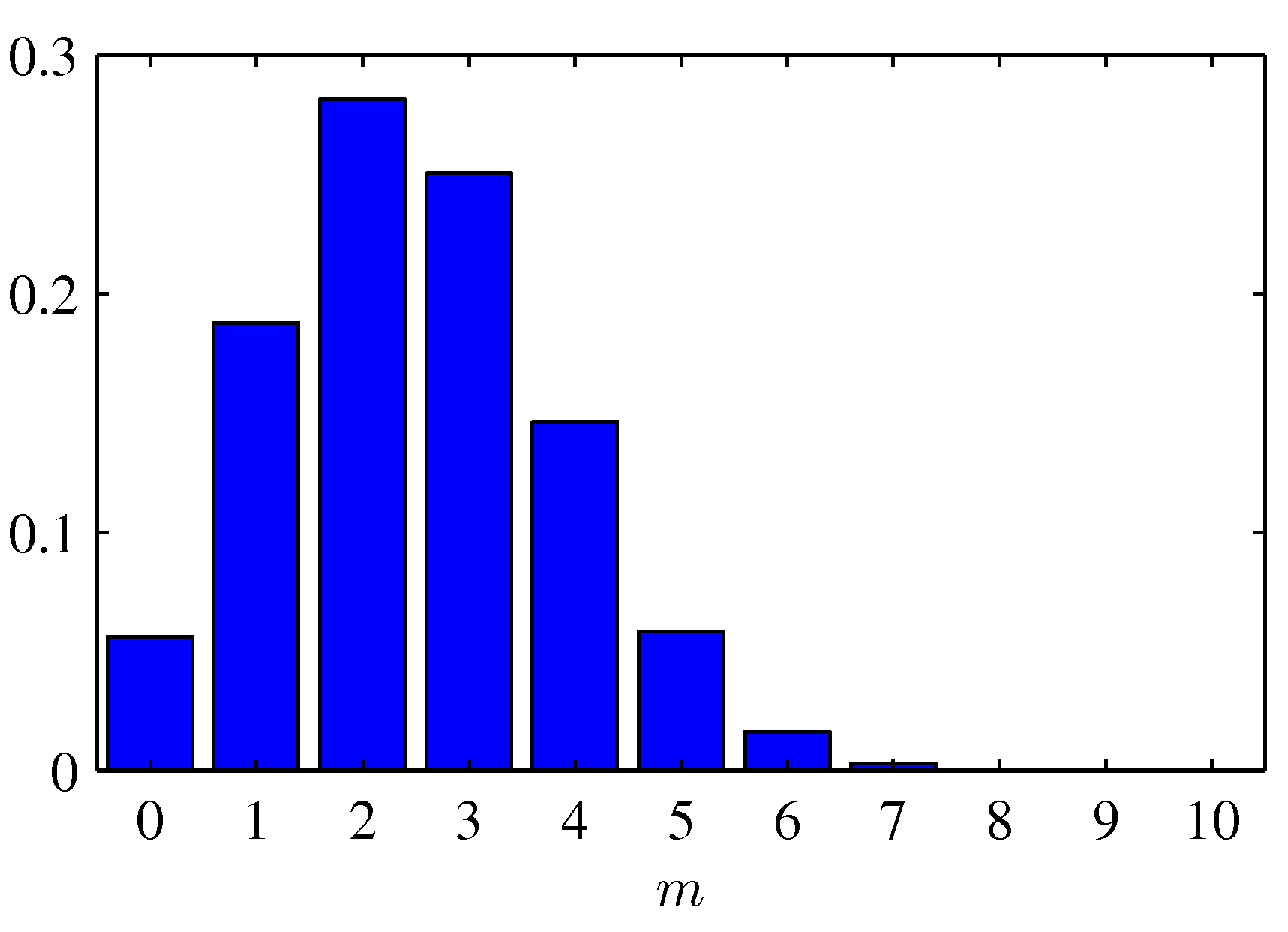
If we only care about the number of heads $m$ in $N$ flips (rather than the order), the count follows a binomial:

\[\operatorname{Bin}(m \mid N, \mu) = \binom{N}{m} \mu^{m} (1 - \mu)^{N - m}. \tag{2.3}\]

Mean and variance: $\mathbb{E}[m] = N\mu$, $\operatorname{var}[m] = N \mu (1 - \mu)$.

Bayesian treatment — the Beta prior

To regularize the MLE on small datasets we put a prior on $\mu$. The Beta distribution

\[\operatorname{Beta}(\mu \mid a, b) = \frac{\Gamma(a + b)}{\Gamma(a)\,\Gamma(b)} \, \mu^{a - 1} (1 - \mu)^{b - 1} \tag{2.4}\]

is the natural choice because its functional form $\mu^{\bullet}(1 - \mu)^{\bullet}$ matches the Bernoulli likelihood. Multiplying the Beta prior by a Bernoulli likelihood gives another Beta — that’s what conjugate means.

Beta distribution shapes — **Fig 2.1.** The Beta distribution for various $a, b$. Setting $a = b$ gives a symmetric distribution; $a > 1, b > 1$ peaks in the interior; $a < 1$ or $b < 1$ pushes mass toward the endpoints.

Mean of the Beta: $\mathbb{E}[\mu] = a / (a + b)$. Variance: $a b / [(a + b)^2 (a + b + 1)]$.

Posterior update

Observing $m$ heads and $\ell = N - m$ tails:

\[p(\mu \mid m, \ell, a, b) \propto \mu^{m + a - 1} (1 - \mu)^{\ell + b - 1}.\]

This is $\operatorname{Beta}(\mu \mid a + m,\, b + \ell)$. The hyperparameters $a$ and $b$ act as pseudocounts — phantom heads and tails that you’re effectively adding to your real observations before computing the proportion.

The posterior mean is

\[\mathbb{E}[\mu \mid \mathcal{D}] = \frac{m + a}{m + a + \ell + b}.\]

In the small-$N$ limit, this is dominated by the prior; in the large-$N$ limit, by the data. The transition is automatic — no manually tuned regularizer.

Sequential learning

Because the posterior has the same shape as the prior, we can update one observation at a time:

\[\operatorname{Beta}(\mu \mid a, b) \xrightarrow{\text{flip lands heads}} \operatorname{Beta}(\mu \mid a + 1,\, b).\]

This is equivalent to one batch update with all observations seen at once — the order doesn’t matter. Useful for streaming or online learning.

2.2 Multinomial Variables

Generalize from two outcomes to $K$ — say drawing one item from a set of $K$ categories. Encode the outcome as a one-hot vector $\mathbf{x} \in \lbrace 0, 1\rbrace^{K}$ with $\sum_k x_k = 1$.

The categorical distribution

If $p(x_k = 1) = \mu_k$ with $\sum_k \mu_k = 1$, then

\[p(\mathbf{x} \mid \boldsymbol{\mu}) = \prod_{k=1}^{K} \mu_k^{x_k}. \tag{2.5}\]

For an i.i.d. dataset $\lbrace \mathbf{x}_n\rbrace_{n=1}^{N}$, the likelihood is

\[p(\mathcal{D} \mid \boldsymbol{\mu}) = \prod_{k=1}^{K} \mu_k^{m_k}, \qquad m_k = \sum_{n=1}^{N} x_{nk}.\]

The sufficient statistics are the per-category counts $\lbrace m_k\rbrace$. Maximizing $\ln p$ subject to $\sum_k \mu_k = 1$ via a Lagrange multiplier gives

\[\mu_{k,\,\mathrm{ML}} = \frac{m_k}{N}.\]

The multinomial distribution

If we just want the joint distribution of the counts $(m_1, \ldots, m_K)$:

\[\operatorname{Mult}(m_1, \ldots, m_K \mid N, \boldsymbol{\mu}) = \binom{N}{m_1\, m_2\, \cdots\, m_K} \prod_{k=1}^{K} \mu_k^{m_k}, \tag{2.6}\]

with $\binom{N}{m_1 \cdots m_K} = N! / \prod_k m_k!$ the multinomial coefficient.

The Dirichlet prior

The multivariate analog of the Beta is the Dirichlet:

\[\operatorname{Dir}(\boldsymbol{\mu} \mid \boldsymbol{\alpha}) = \frac{\Gamma(\alpha_0)}{\prod_k \Gamma(\alpha_k)} \prod_{k=1}^{K} \mu_k^{\alpha_k - 1}, \qquad \alpha_0 = \sum_k \alpha_k. \tag{2.7}\]

It lives on the simplex — the set of probability vectors. Each $\alpha_k$ is a per-category pseudocount.

Dirichlet on simplex — **Fig 2.5.** The Dirichlet distribution over a 3-class simplex for various $\boldsymbol{\alpha}$. Symmetric $\boldsymbol{\alpha}$ centers mass at the centroid; pushing one $\alpha_k$ up biases toward that corner; $\alpha_k < 1$ pulls mass to the edges.

Posterior after observing counts $\lbrace m_k\rbrace$:

\[p(\boldsymbol{\mu} \mid \mathcal{D}, \boldsymbol{\alpha}) = \operatorname{Dir}(\boldsymbol{\mu} \mid \alpha_1 + m_1,\, \ldots,\, \alpha_K + m_K).\]

Same recipe: prior pseudocounts $\boldsymbol{\alpha}$ get added to observed counts $\boldsymbol{m}$.

2.3 The Gaussian Distribution

The single most-used continuous distribution. Univariate form (re-printed from Ch 1):

\[\mathcal{N}(x \mid \mu, \sigma^{2}) = \frac{1}{\sqrt{2\pi\sigma^{2}}} \exp\\!\left(-\frac{(x - \mu)^2}{2 \sigma^2}\right). \tag{2.8}\]

Multivariate form in $D$ dimensions:

\[\mathcal{N}(\mathbf{x} \mid \boldsymbol{\mu}, \boldsymbol{\Sigma}) = \frac{1}{(2\pi)^{D/2} |\boldsymbol{\Sigma}|^{1/2}} \exp\\!\left(-\tfrac{1}{2} \Delta^{2}\right), \tag{2.9}\]

where

\[\Delta^{2} = (\mathbf{x} - \boldsymbol{\mu})^{\top} \boldsymbol{\Sigma}^{-1} (\mathbf{x} - \boldsymbol{\mu})\]

is the Mahalanobis distance — a generalized squared distance that accounts for correlations and per-dimension scales.

Geometry of the Gaussian

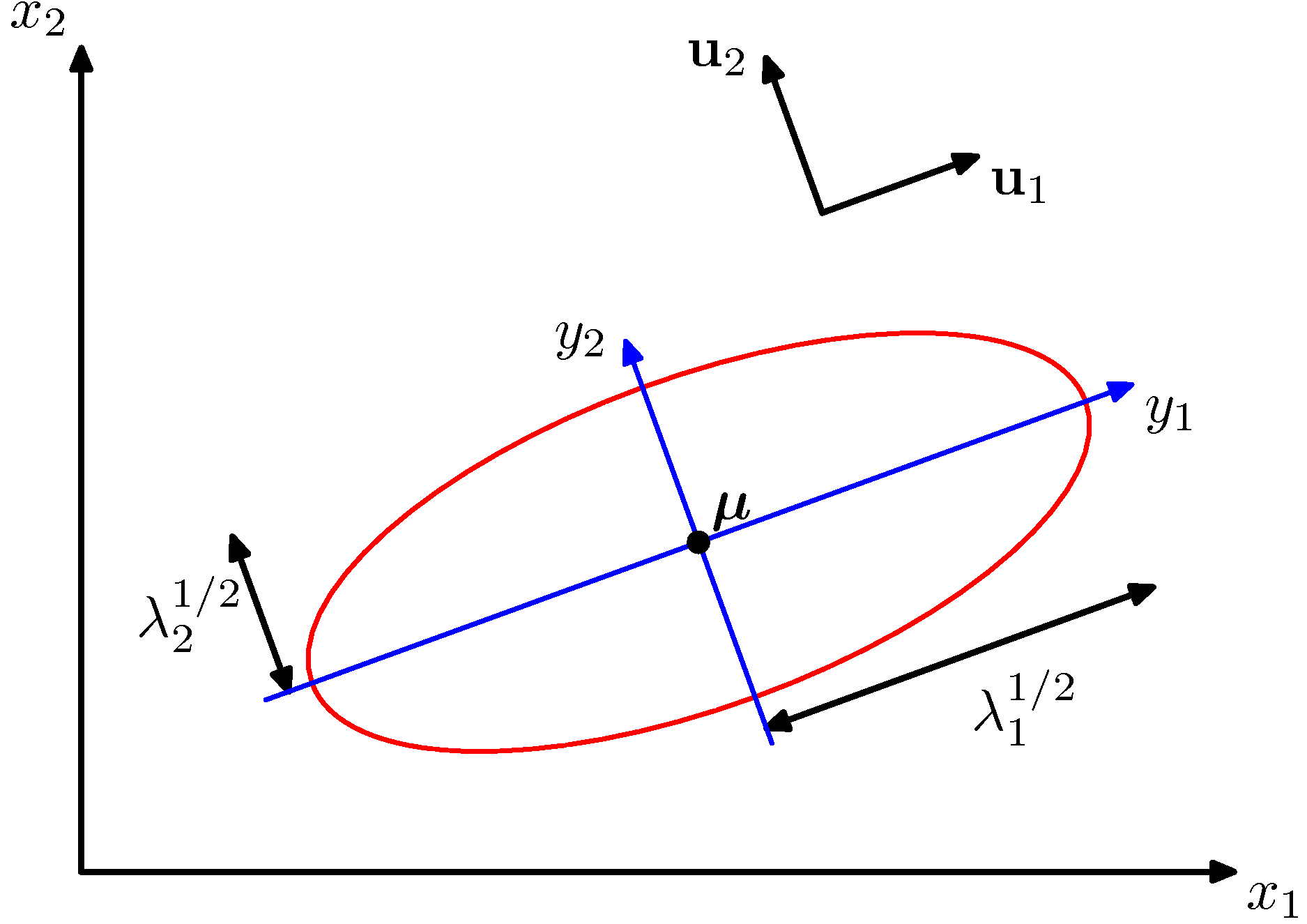
Surfaces of constant density are ellipsoids whose principal axes are the eigenvectors of $\boldsymbol{\Sigma}$, with axis lengths proportional to $\sqrt{\lambda_i}$ (the square-root eigenvalues). Three special cases:

General covariance — ellipsoidal contours with arbitrary orientation and per-axis scale.
Diagonal covariance — ellipsoidal contours aligned with the coordinate axes.
Isotropic ($\boldsymbol{\Sigma} = \sigma^2 \mathbf{I}$) — spherical contours.

Gaussian contours — **Fig 2.7.** Constant-density contours of a 2-D Gaussian under (left) general, (middle) diagonal, and (right) isotropic covariance. Ellipse axes are the eigenvectors of $\boldsymbol{\Sigma}$; axis lengths are $\propto \sqrt{\lambda_i}$.

Why Gaussians appear so often

Two reasons:

Central Limit Theorem. Sums of many independent random variables tend toward Gaussian, regardless of the individual distributions. So measurement noise — which is often a sum of many small effects — is approximately Gaussian.
Maximum entropy. Among all distributions on $\mathbb{R}$ with a given mean and variance, the Gaussian has the largest entropy. Picking a Gaussian commits to as little additional structure as possible given those two moments.

Conditional and marginal Gaussians

Partition $\mathbf{x}$ into $\mathbf{x}_a, \mathbf{x}_b$ with corresponding partitions of $\boldsymbol{\mu}$ and $\boldsymbol{\Sigma}$:

\[\boldsymbol{\mu} = \begin{pmatrix}\boldsymbol{\mu}_a \\ \boldsymbol{\mu}_b\end{pmatrix}, \qquad \boldsymbol{\Sigma} = \begin{pmatrix}\boldsymbol{\Sigma}_{aa} & \boldsymbol{\Sigma}_{ab} \\ \boldsymbol{\Sigma}_{ba} & \boldsymbol{\Sigma}_{bb}\end{pmatrix}.\]

Two closed-form results that get used everywhere:

Marginal: $p(\mathbf{x}_a) = \mathcal{N}(\mathbf{x}_a \mid \boldsymbol{\mu}_a, \boldsymbol{\Sigma}_{aa})$.
Conditional: $p(\mathbf{x}_a \mid \mathbf{x}_b) = \mathcal{N}(\mathbf{x}_a \mid \boldsymbol{\mu}_{a \mid b}, \boldsymbol{\Sigma}_{a \mid b})$ with

\[\begin{aligned} \boldsymbol{\mu}_{a \mid b} &= \boldsymbol{\mu}_a + \boldsymbol{\Sigma}_{ab} \boldsymbol{\Sigma}_{bb}^{-1} (\mathbf{x}_b - \boldsymbol{\mu}_b), \\ \boldsymbol{\Sigma}_{a \mid b} &= \boldsymbol{\Sigma}_{aa} - \boldsymbol{\Sigma}_{ab} \boldsymbol{\Sigma}_{bb}^{-1} \boldsymbol{\Sigma}_{ba}. \end{aligned}\]

Both marginals and conditionals of Gaussians are Gaussian — a property that makes Gaussian models tractable across the board.

Maximum likelihood for the Gaussian

Given $\mathcal{D} = \lbrace \mathbf{x}_1, \ldots, \mathbf{x}_N\rbrace$ i.i.d. from $\mathcal{N}(\boldsymbol{\mu}, \boldsymbol{\Sigma})$, the log-likelihood is

\[\ln p(\mathcal{D} \mid \boldsymbol{\mu}, \boldsymbol{\Sigma}) = -\frac{N D}{2} \ln(2 \pi) - \frac{N}{2} \ln |\boldsymbol{\Sigma}| - \frac{1}{2} \sum_{n=1}^{N} (\mathbf{x}_n - \boldsymbol{\mu})^{\top} \boldsymbol{\Sigma}^{-1} (\mathbf{x}_n - \boldsymbol{\mu}).\]

Differentiating and solving:

\[\boxed{\,\boldsymbol{\mu}_{\mathrm{ML}} = \frac{1}{N} \sum_{n=1}^{N} \mathbf{x}_n, \qquad \boldsymbol{\Sigma}_{\mathrm{ML}} = \frac{1}{N} \sum_{n=1}^{N} (\mathbf{x}_n - \boldsymbol{\mu}_{\mathrm{ML}}) (\mathbf{x}_n - \boldsymbol{\mu}_{\mathrm{ML}})^{\top}.\,} \tag{2.10}\]

The mean MLE is unbiased; the covariance MLE is biased low by a factor of $(N-1)/N$. The bias-corrected estimator divides by $N - 1$ instead — this is what statistics packages call “sample variance.”

Sequential learning and the Robbins–Monro algorithm

A useful identity: writing the running mean recursively,

\[\boldsymbol{\mu}_{\mathrm{ML}}^{(N)} = \boldsymbol{\mu}_{\mathrm{ML}}^{(N-1)} + \frac{1}{N}\bigl(\mathbf{x}_N - \boldsymbol{\mu}_{\mathrm{ML}}^{(N-1)}\bigr).\]

This is the prototype for stochastic gradient updates: each step nudges the estimate toward the new observation, with a step size that decays as $1/N$. The Robbins–Monro algorithm generalizes this to any objective whose gradient can be written as an expectation.

2.4 The Exponential Family

All the distributions above (Bernoulli, multinomial, Gaussian, plus exponential, Poisson, Beta, Dirichlet, gamma…) are special cases of a single family with a unified theory. A distribution is in the exponential family if it can be written as

\[p(\mathbf{x} \mid \boldsymbol{\eta}) = h(\mathbf{x})\, g(\boldsymbol{\eta})\, \exp\bigl( \boldsymbol{\eta}^{\top} \mathbf{u}(\mathbf{x}) \bigr), \tag{2.11}\]

where:

$\boldsymbol{\eta}$ — the natural parameters. (2.11) is linear in them inside the exponent.
$\mathbf{u}(\mathbf{x})$ — the sufficient statistics. All the data tells you about $\boldsymbol{\eta}$ is summarized by $\sum_n \mathbf{u}(\mathbf{x}_n)$.
$h(\mathbf{x})$ — a non-negative base measure.
$g(\boldsymbol{\eta})$ — the partition function ensuring $p$ integrates to 1.

Why the exponential family is worth knowing

Three universal facts that come for free once you’ve cast a model in this form:

MLE is solving a moment-matching equation. The MLE for $\boldsymbol{\eta}$ satisfies
\[-\nabla \ln g(\boldsymbol{\eta}) = \frac{1}{N} \sum_{n=1}^{N} \mathbf{u}(\mathbf{x}_n),\]
i.e. set the model’s expected sufficient statistic equal to the empirical one.
Conjugate priors always exist (and have a known form) for any exponential-family likelihood. That’s why Bernoulli has Beta, Gaussian has Gaussian, multinomial has Dirichlet — they’re not coincidences.
Maximum-entropy derivation. Many exponential-family distributions are the maximum-entropy distribution subject to specific moment constraints (mean only → exponential; mean and variance → Gaussian; etc.).

We won’t derive the partition function for every example, but in chapters 8–11 (when we hit graphical models and variational inference) the exponential-family viewpoint becomes essential.

2.5 Nonparametric Methods

When no parametric family is appropriate — say the density is multimodal in a way no Gaussian mixture captures cleanly — we fall back on nonparametric methods. Two families:

Histograms and kernel density estimation (KDE). Place a small “bump” (the kernel) on each data point and average. Bandwidth is the regularization knob; too small and you overfit, too large and you smear out structure.
K-nearest-neighbours. Density at $\mathbf{x}$ is estimated as $K / (NV)$, where $V$ is the volume of the smallest sphere around $\mathbf{x}$ that contains $K$ training points. Same overfitting/underfitting trade-off in $K$.

These are useful diagnostics and baselines, but they scale poorly with dimension — densities in $\mathbb{R}^{D}$ require exponentially more data as $D$ grows. We mostly stick with parametric methods from chapter 3 onward.

Takeaways

Bernoulli ↔ Beta and Multinomial ↔ Dirichlet: the prior pseudocounts add to data counts; the posterior mean smoothly interpolates between prior and ML.
The Gaussian’s tractability — closed-form marginals, conditionals, MLEs, and conjugate priors — is the reason it appears in every later chapter.
The exponential family unifies all of the above. Once a model is in standard form, MLE recipes and conjugate priors fall out automatically.
Nonparametric methods are useful for low-dimensional density estimation and as sanity checks, but suffer the curse of dimensionality.

Forward to Ch 3 — Linear Models for Regression, where we generalize the polynomial fit of Ch 1 to arbitrary basis functions and develop the full Bayesian treatment.

Figures from Bishop, Pattern Recognition and Machine Learning (Springer, 2006), © Springer / C. M. Bishop. Reproduced for educational use.