Ch 1 — Introduction

Machine learning sits at the intersection of statistics, optimization, and computer science. Given experience in the form of data, the goal is to make good predictions about quantities of interest. The classic motivating example is automatic recognition of handwritten digits: each image is represented by a vector of pixel intensities \(\mathbf{x} \in \mathbb{R}^{D}\), and the task is to predict the correct label \(t \in \lbrace 0, 1, \ldots, 9\rbrace \). Rather than hand-coding rules for every quirk of human handwriting, ML methods learn these rules from a large collection of labeled examples.

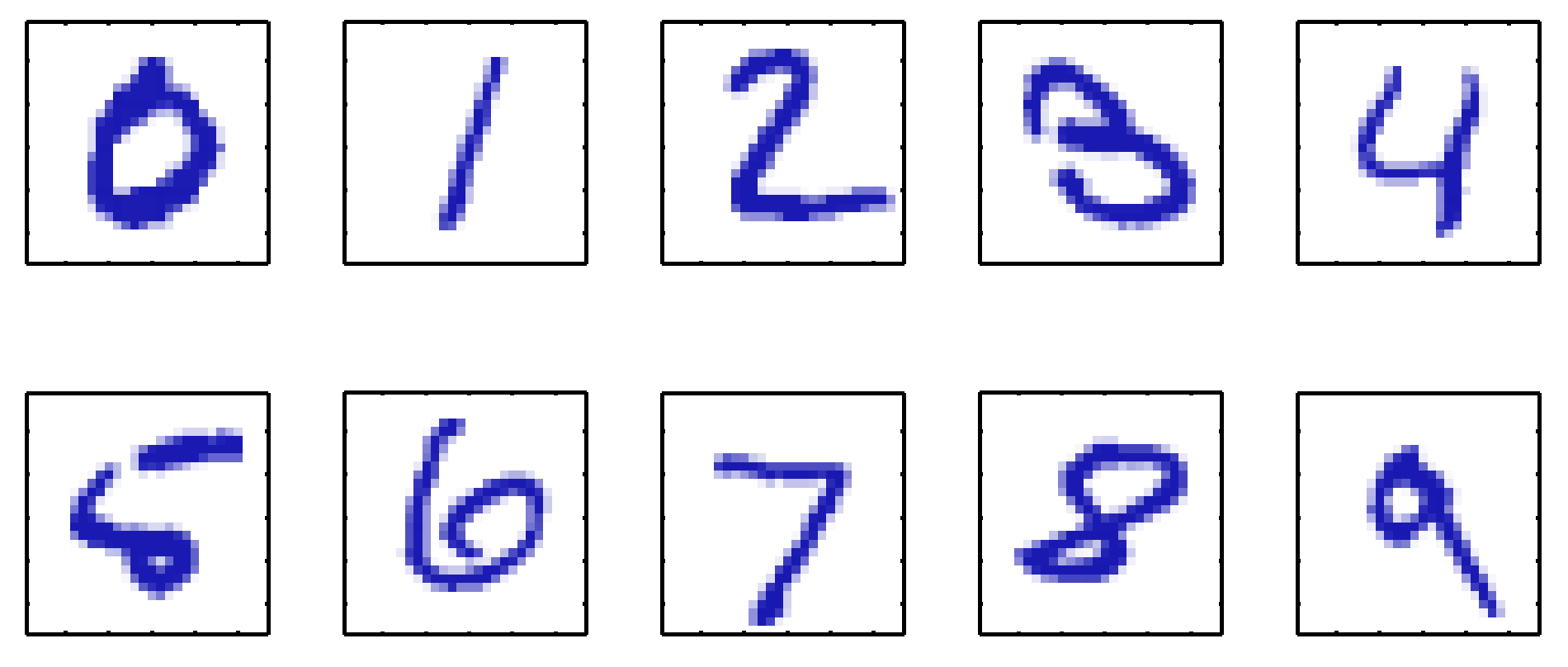
ML problems are traditionally grouped into three paradigms by the structure of the training data and the feedback the learner receives:

Paradigm	Training data	Goal	Examples
Supervised	Inputs \(\mathbf{x}_n\) paired with targets \(t_n\)	Classification (discrete \(t\)); regression (continuous \(t\))	Digit recognition, chemical-yield prediction
Unsupervised	Inputs \(\mathbf{x}_n\) only — no targets	Clustering, density estimation, dimensionality reduction	Grouping similar examples, 2-D data embeddings
Reinforcement	States, actions, scalar rewards from interacting with an environment	Maximize cumulative reward; resolve credit-assignment and exploration–exploitation tradeoffs	Game-playing agents, robotic control

Prerequisites for this chapter

• Linear algebra: vectors, dot product, matrix–vector multiplication, transpose, matrix inverse.
• Calculus: partial derivatives and the gradient. To minimize a sum of squares we’ll set \(\partial / \partial w_j = 0\).
• Probability: the sum and product rules; what a probability density is. We re-derive the rest below from scratch.

If any of these feel rusty, skim a refresher before reading on.

---

1.1 Example — Polynomial Curve Fitting

We begin with a concrete regression example that runs through the chapter. Suppose we observe a training set of \(N = 10\) points \(\lbrace (x_n, t_n)\rbrace _{n=1}^{N}\), where each input \(x_n\) is drawn from \([0, 1]\) and the target is generated by

\[t_n = \sin(2\pi x_n) + \epsilon_n, \qquad \epsilon_n \sim \mathcal{N}(0, \sigma^2).\]

Here \(\mathcal{N}(0, \sigma^2)\) denotes a Gaussian (normal) distribution with mean \(0\) and variance \(\sigma^2\). The noise term \(\epsilon_n\) models the fact that real measurements are never perfect.

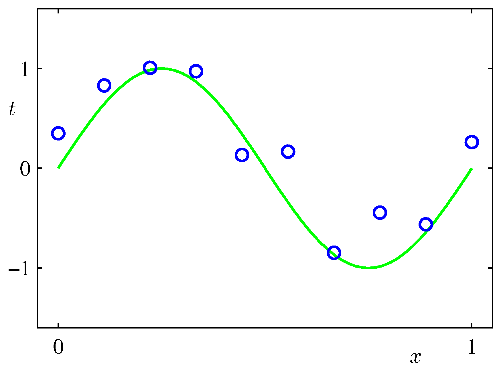
Our goal is to predict \(t\) at a new input \(x\) without knowing the generating function in advance. We must learn it from the data alone.

A polynomial model

One simple class of models is a polynomial in \(x\):

\[y(x, \mathbf{w}) = w_0 + w_1 x + w_2 x^2 + \cdots + w_M x^M = \sum_{j=0}^{M} w_j x^{j}. \tag{1.1}\]

Read the symbols carefully:

• \(M\) is the order of the polynomial — a hyperparameter we choose.
• \(\mathbf{w} = (w_0, w_1, \ldots, w_M)^{\top}\) is the parameter vector. The superscript \(\top\) denotes transpose, so \(\mathbf{w}\) is a column vector of length \(M+1\).
• \(y(x, \mathbf{w})\) is the model’s prediction at input \(x\) given parameters \(\mathbf{w}\).

A subtle but important point: although \(y\) is non-linear in \(x\) (because of the powers), it is linear in \(\mathbf{w}\). Models that are linear in their parameters are called linear models, and they have a unique global minimum for sum-of-squares objectives — so curve fitting reduces to solving a linear system.

Sum-of-squares error

We need to choose \(\mathbf{w}\) so that \(y(x_n, \mathbf{w})\) is close to \(t_n\) for every training point. The natural way to measure “closeness” is the sum-of-squares error

\[E(\mathbf{w}) = \frac{1}{2} \sum_{n=1}^{N} \bigl\lbrace y(x_n, \mathbf{w}) - t_n \bigr\rbrace ^{2}. \tag{1.2}\]

The factor of \(\tfrac{1}{2}\) is purely cosmetic — it cancels the 2 from the chain rule when we differentiate. The squared difference \((y - t)^2\) penalizes both over- and under-shooting equally and grows quickly as the gap widens.

Solving for the optimum

To minimize \(E(\mathbf{w})\), set its partial derivatives to zero:

\[\frac{\partial E}{\partial w_j} = \sum_{n=1}^{N} \bigl\lbrace y(x_n, \mathbf{w}) - t_n \bigr\rbrace \, x_n^{j} = 0, \qquad j = 0, 1, \ldots, M.\]

Substituting \(y(x_n, \mathbf{w}) = \sum_i w_i x_n^{i}\) and rearranging gives the normal equations:

\[\sum_{i=0}^{M} A_{ji}\, w_i = T_j, \qquad A_{ji} = \sum_{n=1}^{N} x_n^{j+i}, \quad T_j = \sum_{n=1}^{N} x_n^{j}\, t_n. \tag{1.3}\]

These are \(M+1\) linear equations in the \(M+1\) unknowns \(w_0, \ldots, w_M\). In matrix form, \(\mathbf{A}\mathbf{w} = \mathbf{t}\), with the unique solution \(\mathbf{w}^{\star} = \mathbf{A}^{-1}\mathbf{t}\) (assuming \(\mathbf{A}\) is invertible). Crucially, no iterative optimization is needed: a single linear solve gives the answer.

Choosing the model order \(M\)

Different choices of \(M\) produce qualitatively different fits.

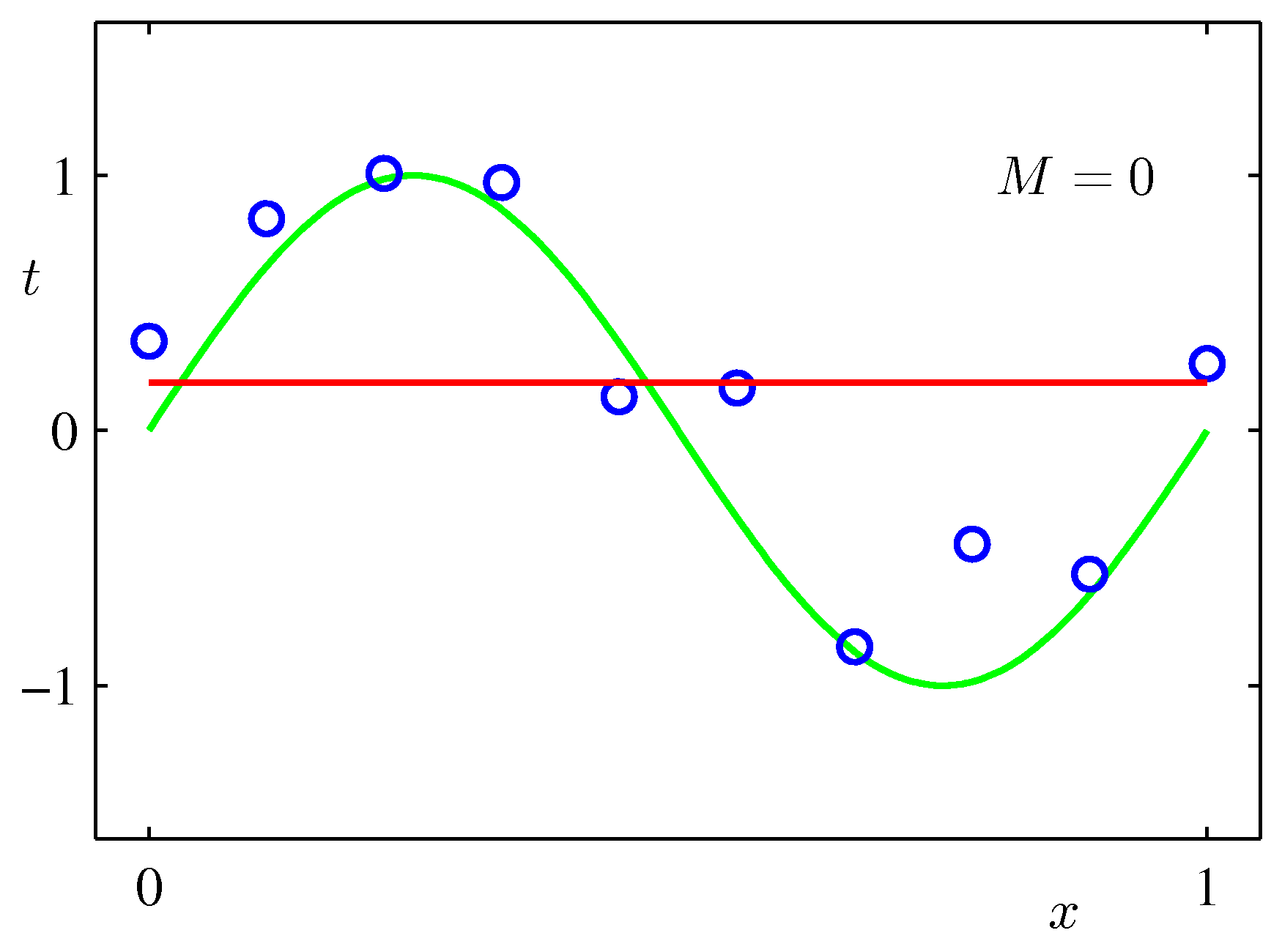
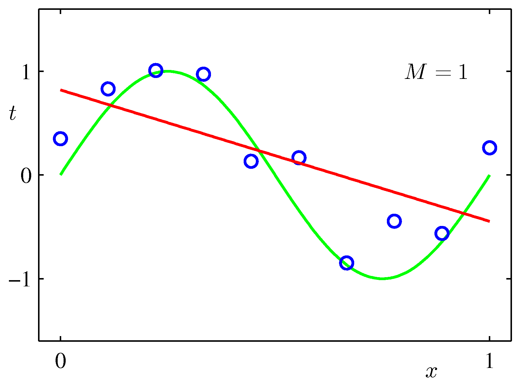
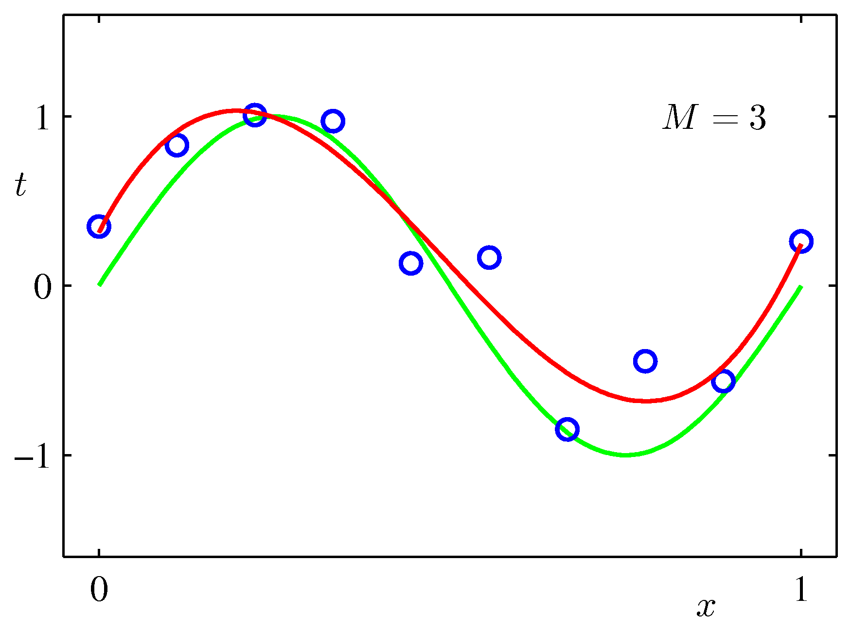
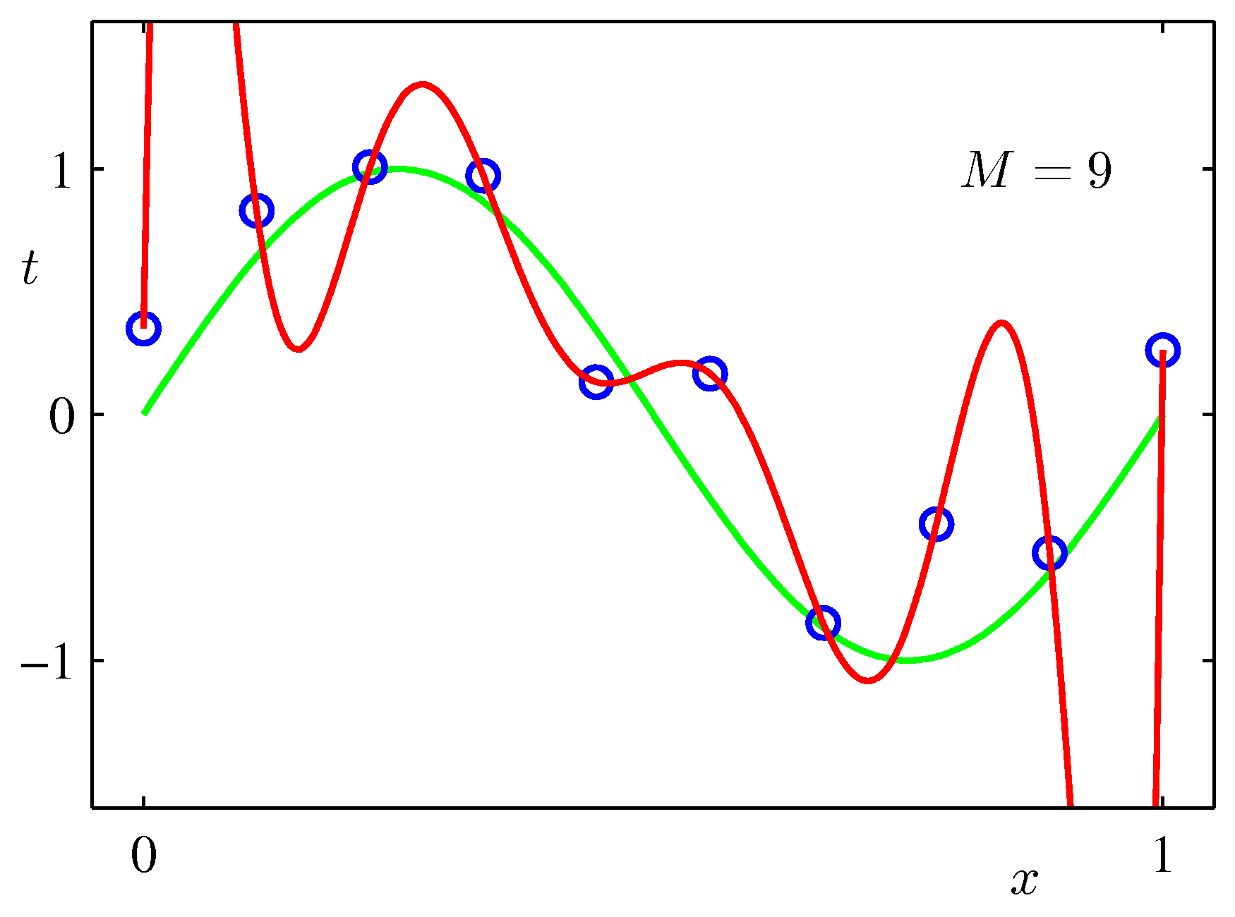
This is overfitting: a model with enough capacity (\(M \geq N - 1\)) can match every training point, but at the cost of producing absurd predictions in between. The fitted weights \(\mathbf{w}^{\star}\) also blow up — for \(M=9\) on this dataset they can be on the order of \(10^{5}\), with alternating signs that almost cancel.

Quantifying generalization

To compare \(M\) values fairly, draw a fresh test set of 100 points from the same generating process and compute the root-mean-square error

\[E_{\mathrm{RMS}} = \sqrt{\, 2 E(\mathbf{w}^{\star}) / N \,}. \tag{1.4}\]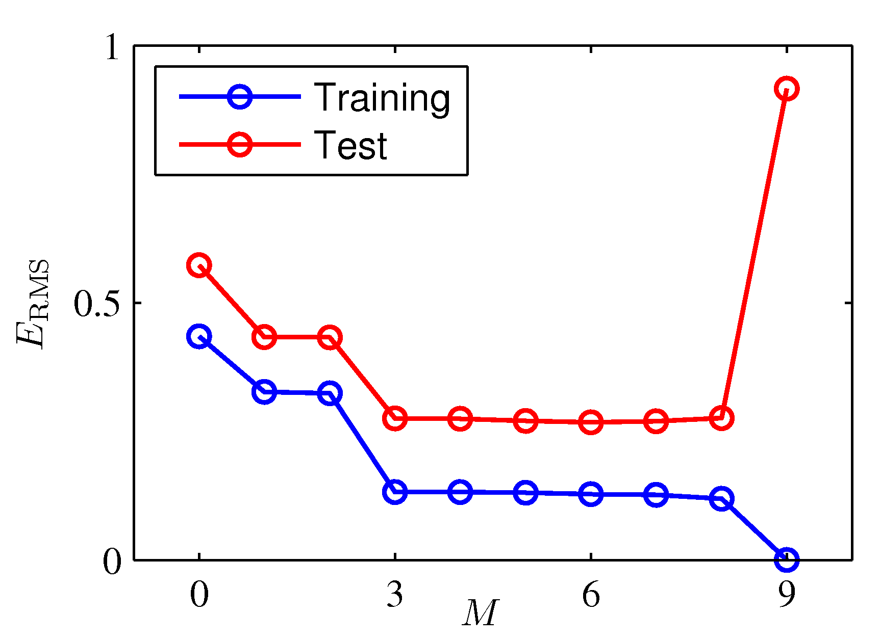

The right \(M\) lives in the dip — small enough to avoid overfitting, large enough to express the data’s shape.

Effect of the dataset size

A second way to fight overfitting is more data.

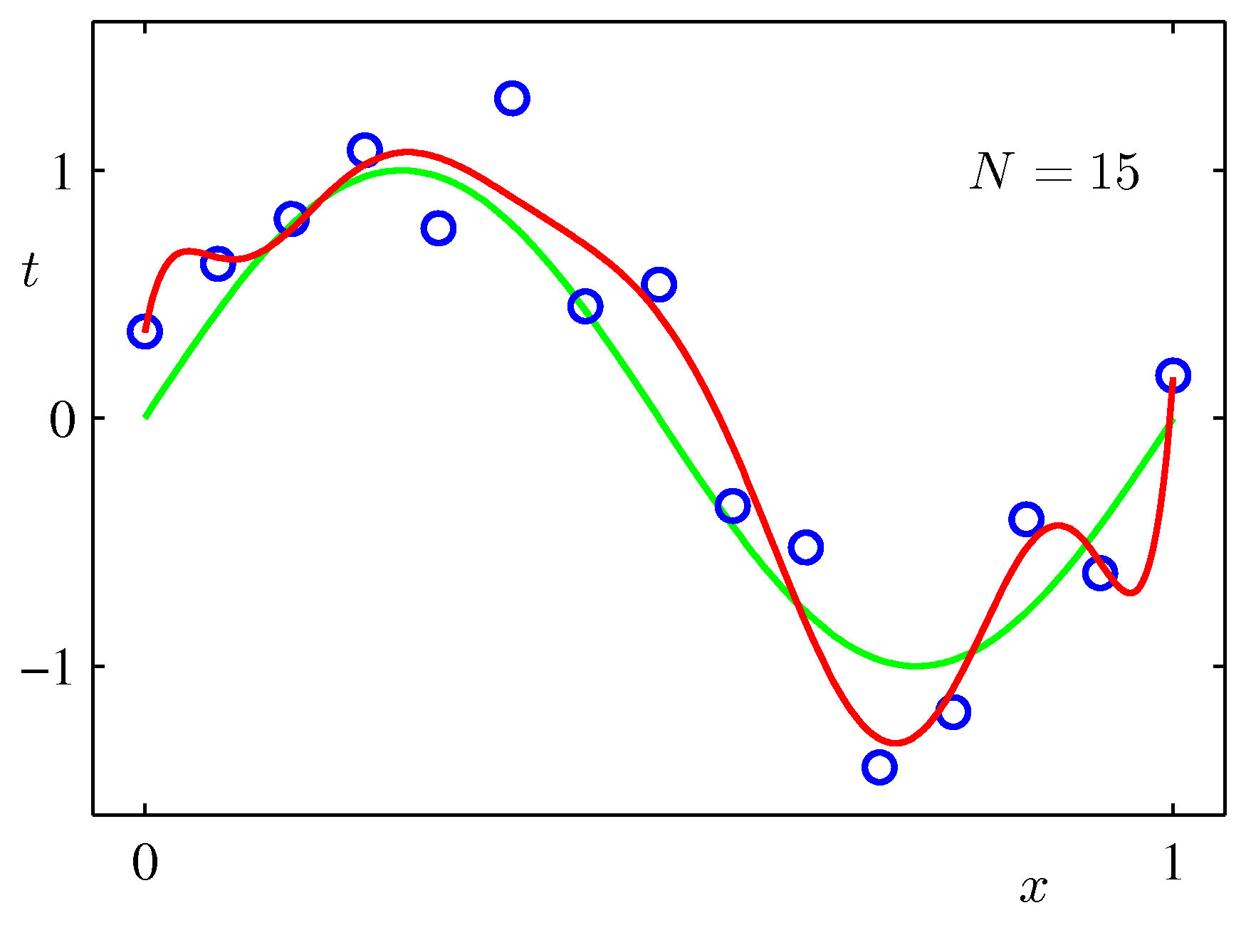
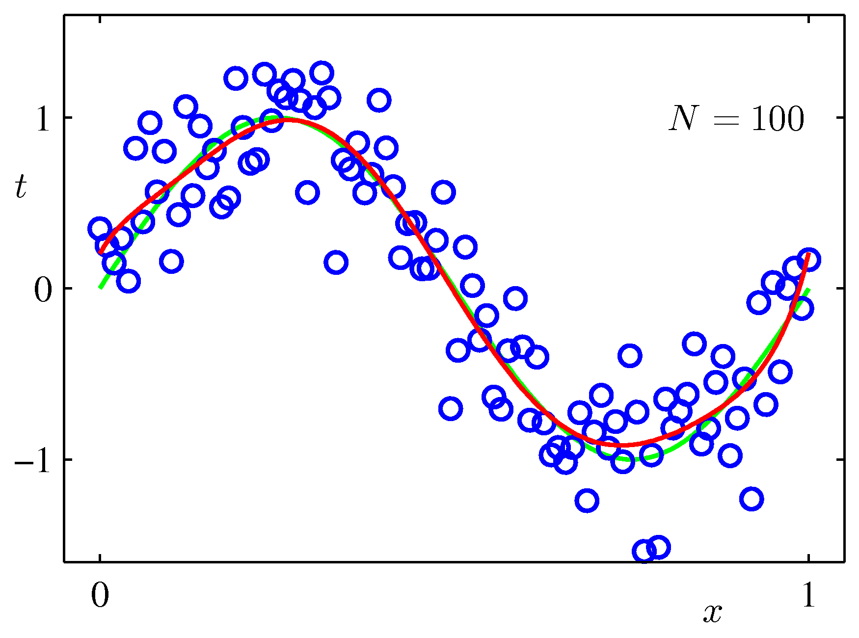
We’ll see in §1.2 that Bayesian methods make this rule unnecessary by automatically adapting model complexity.

Regularization

A third lever is to penalize large weights directly. Define

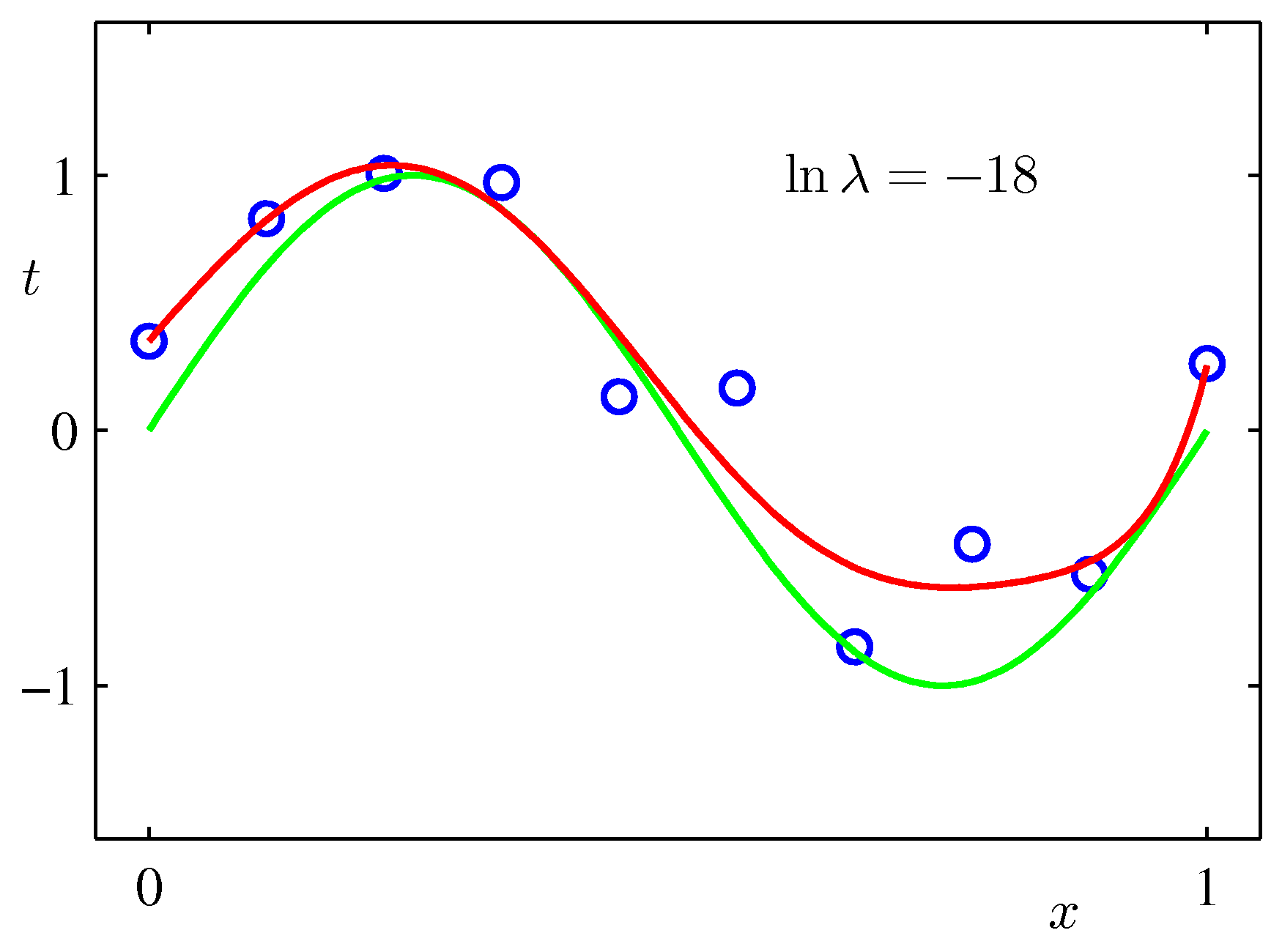
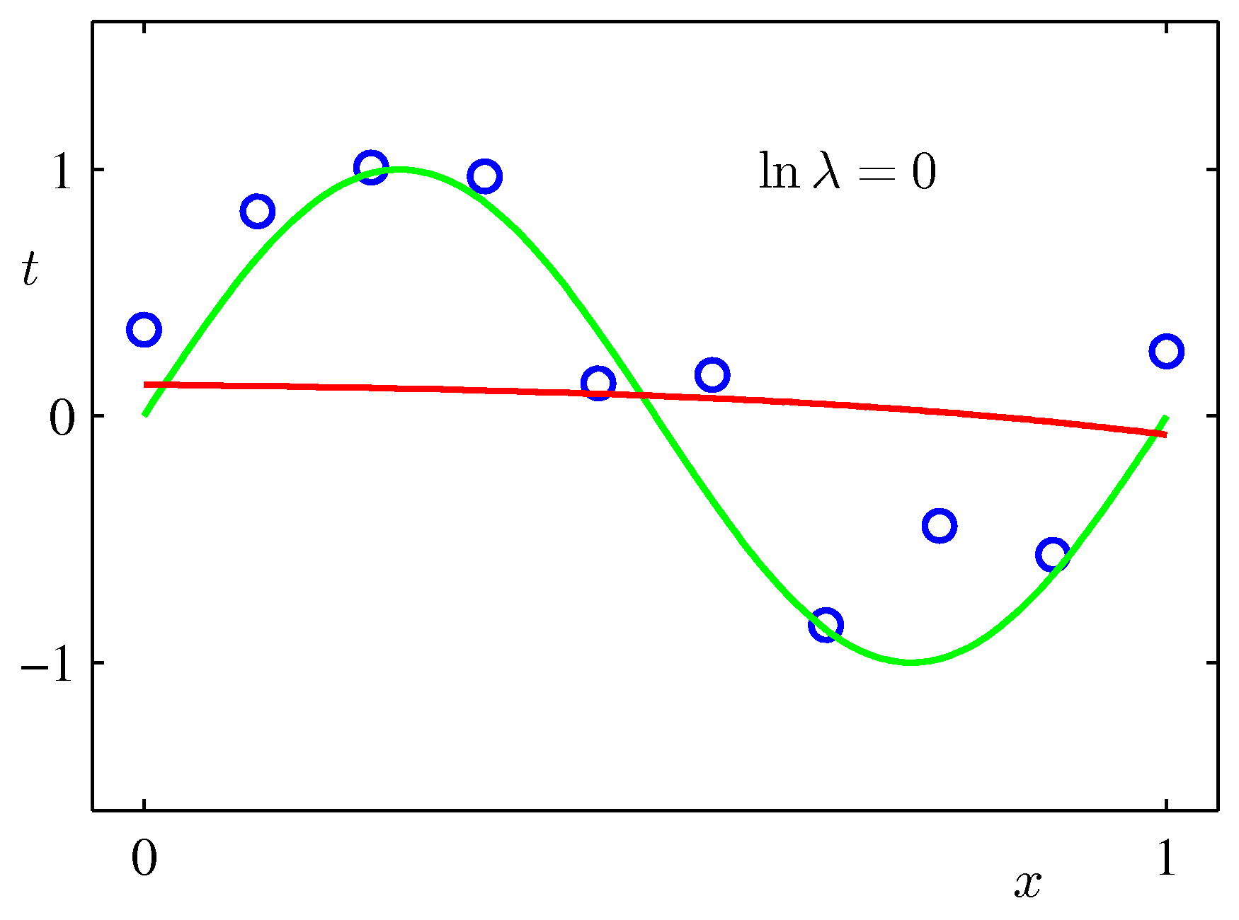
\[\widetilde{E}(\mathbf{w}) = \frac{1}{2} \sum_{n=1}^{N} \lbrace y(x_n, \mathbf{w}) - t_n\rbrace ^{2} + \frac{\lambda}{2} \, \|\mathbf{w}\|^{2}, \tag{1.5}\]

where \(\|\mathbf{w}\|^{2} = \mathbf{w}^{\top}\mathbf{w} = \sum_j w_j^{2}\) and \(\lambda \geq 0\) is the regularization strength (a hyperparameter). The added term \(\tfrac{\lambda}{2}\|\mathbf{w}\|^2\) pushes the weights toward zero.

• \(\lambda = 0\) recovers the unregularized fit.
• \(\lambda \to \infty\) forces all \(w_j \to 0\), returning a flat function.
• Intermediate \(\lambda\) trades off fit vs. weight magnitude.

In statistics this technique is called ridge regression (and goes by shrinkage more generally). In neural networks it’s often called weight decay, because each gradient step shrinks \(\mathbf{w}\) slightly toward zero before moving in the data direction.

The regularized normal equations are

\[(\mathbf{A} + \lambda \mathbf{I})\, \mathbf{w} = \mathbf{t}. \tag{1.6}\]

Adding \(\lambda \mathbf{I}\) to the diagonal of \(\mathbf{A}\) also makes the matrix easier to invert numerically — even when the unregularized \(\mathbf{A}\) is nearly singular, \(\mathbf{A} + \lambda \mathbf{I}\) is well-conditioned for any \(\lambda > 0\).

---

1.2 Probability Theory

A central theme in PRML is that probability is the right language for handling uncertainty — both noise in the data and incomplete knowledge about the model. We re-derive the basic rules here.

Sum and product rules

Imagine two random variables \(X\) and \(Y\). Let \(p(X=x_i, Y=y_j)\) denote the joint probability that \(X = x_i\) and \(Y = y_j\). Then:

\[\boxed{\;p(X=x_i) = \sum_j p(X=x_i, Y=y_j)\;} \quad\text{(sum rule, marginalization)}\] \[\boxed{\;p(X=x_i, Y=y_j) = p(Y=y_j \mid X=x_i)\, p(X=x_i)\;} \quad\text{(product rule)}\]

The conditional probability \(p(Y \mid X)\) reads “probability of \(Y\) given \(X\).” Combining the two yields Bayes’ theorem:

\[\boxed{\;p(Y \mid X) = \frac{p(X \mid Y)\, p(Y)}{p(X)}\;} \tag{1.7}\]

with \(p(X) = \sum_Y p(X \mid Y)\, p(Y)\) in the denominator (the sum rule applied to make the right-hand side a valid probability).

In ML, Bayes’ theorem is the bridge between models and data. Treating the parameters \(\mathbf{w}\) as a random variable:

\[p(\mathbf{w} \mid \mathcal{D}) = \frac{p(\mathcal{D} \mid \mathbf{w})\, p(\mathbf{w})}{p(\mathcal{D})}\]

• \(p(\mathbf{w})\) — the prior — what we believed about \(\mathbf{w}\) before seeing data.
• \(p(\mathcal{D} \mid \mathbf{w})\) — the likelihood — how probable the data is given \(\mathbf{w}\).
• \(p(\mathbf{w} \mid \mathcal{D})\) — the posterior — what we should believe after seeing the data.
• \(p(\mathcal{D})\) — the evidence (a normalization constant).

Probability densities

For continuous variables, replace probabilities of values with densities. A probability density \(p(x)\) satisfies \(p(x) \geq 0\) and \(\int p(x)\,\mathrm{d}x = 1\), and the probability that \(x\) lies in \([a, b]\) is \(\int_a^b p(x)\,\mathrm{d}x\). Sum and product rules continue to hold, with sums replaced by integrals.

Expectation and variance

The expectation of a function \(f(x)\) under \(p(x)\) is

\[\mathbb{E}[f] = \sum_x p(x) f(x) \quad\text{or}\quad \mathbb{E}[f] = \int p(x) f(x)\,\mathrm{d}x. \tag{1.8}\]

The variance measures spread:

\[\operatorname{var}[f] = \mathbb{E}\bigl[(f(x) - \mathbb{E}[f])^{2}\bigr] = \mathbb{E}[f(x)^{2}] - \mathbb{E}[f(x)]^{2}. \tag{1.9}\]

For two variables, the covariance is \(\operatorname{cov}[x, y] = \mathbb{E}\bigl[(x - \mathbb{E}[x])(y - \mathbb{E}[y])\bigr]\).

The Gaussian distribution

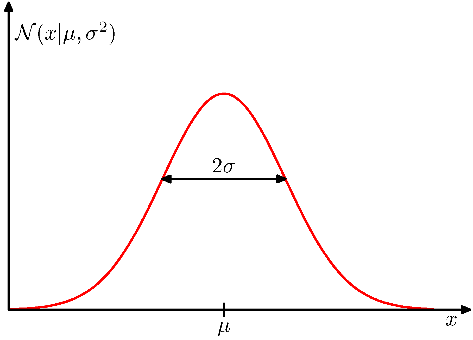
The single most-used distribution. In one dimension,

\[\mathcal{N}(x \mid \mu, \sigma^{2}) = \frac{1}{\sqrt{2\pi\sigma^{2}}} \exp\\!\left(-\frac{(x - \mu)^{2}}{2\sigma^{2}}\right) \tag{1.10}\]

with \(\mathbb{E}[x] = \mu\), \(\operatorname{var}[x] = \sigma^{2}\). The reciprocal \(\beta = 1/\sigma^{2}\) is called the precision.

In \(D\) dimensions, with mean vector \(\boldsymbol{\mu}\) and covariance matrix \(\boldsymbol{\Sigma}\),

\[\mathcal{N}(\mathbf{x} \mid \boldsymbol{\mu}, \boldsymbol{\Sigma}) = \frac{1}{(2\pi)^{D/2} |\boldsymbol{\Sigma}|^{1/2}} \exp\\!\left(-\tfrac{1}{2} (\mathbf{x} - \boldsymbol{\mu})^{\top} \boldsymbol{\Sigma}^{-1} (\mathbf{x} - \boldsymbol{\mu})\right). \tag{1.11}\]

Curve fitting, revisited probabilistically

The polynomial-fit setup gets a clean Bayesian re-cast. Assume the targets are Gaussian-perturbed versions of the model output:

\[p(t \mid x, \mathbf{w}, \beta) = \mathcal{N}(t \mid y(x, \mathbf{w}), \beta^{-1}).\]

For an i.i.d. dataset \(\lbrace (x_n, t_n)\rbrace \), the likelihood is

\[p(\mathbf{t} \mid \mathbf{x}, \mathbf{w}, \beta) = \prod_{n=1}^{N} \mathcal{N}(t_n \mid y(x_n, \mathbf{w}), \beta^{-1}).\]

Taking the logarithm and dropping terms that don’t depend on \(\mathbf{w}\):

\[\ln p(\mathbf{t} \mid \mathbf{x}, \mathbf{w}, \beta) = -\frac{\beta}{2} \sum_{n=1}^{N} \lbrace y(x_n, \mathbf{w}) - t_n\rbrace ^{2} + \frac{N}{2} \ln \beta - \frac{N}{2} \ln(2\pi).\]

Maximizing the log-likelihood with respect to \(\mathbf{w}\) is equivalent to minimizing the sum-of-squares error (1.2). The Gaussian-noise model is what justifies sum-of-squares as the loss.

Adding a Gaussian prior \(p(\mathbf{w} \mid \alpha) = \mathcal{N}(\mathbf{w} \mid \mathbf{0}, \alpha^{-1}\mathbf{I})\) and taking the log of the posterior reproduces the regularized objective (1.5), with \(\lambda = \alpha / \beta\). So ridge regression is the maximum a posteriori (MAP) estimate under a Gaussian prior on \(\mathbf{w}\).

Predictive distribution

A fully Bayesian treatment goes one step further: instead of picking a single best \(\mathbf{w}\), integrate over the posterior

\[p(t \mid x, \mathcal{D}) = \int p(t \mid x, \mathbf{w}) \, p(\mathbf{w} \mid \mathcal{D}) \, \mathrm{d}\mathbf{w}.\]

For the Gaussian-noise polynomial fit, this integral is tractable (Gaussian × Gaussian is Gaussian) and yields a predictive distribution whose variance grows as \(x\) moves away from training points — a quantitative measure of the model’s uncertainty. We’ll redo this carefully in chapter 3.

---

1.3 Decision Theory

Probability lets us describe uncertainty; decision theory tells us how to act on it.

In a classification problem with classes \(\mathcal{C}_k\), after computing the posterior \(p(\mathcal{C}_k \mid \mathbf{x})\) via Bayes’ theorem we still have to commit to a single predicted class. Decision theory says: pick the class that minimizes the expected loss under the posterior.

Loss matrices

Define a loss matrix \(L_{kj}\) — the cost of predicting class \(j\) when the true class is \(k\). The expected loss for predicting class \(j\) on input \(\mathbf{x}\) is

\[\mathbb{E}[L \mid \mathbf{x}, \text{pred} = j] = \sum_k L_{kj}\, p(\mathcal{C}_k \mid \mathbf{x}).\]

The optimal decision picks \(j\) to minimize this. For the special case \(L_{kj} = 1 - \delta_{kj}\) (zero-one loss — penalize every misclassification equally), this reduces to predicting the class with the highest posterior probability.

The reject option

If no class has high enough posterior probability — say \(\max_k p(\mathcal{C}_k \mid \mathbf{x}) < \theta\) — we may want the system to abstain. This is sensible in safety-critical applications (medical diagnosis, fraud detection): better to flag uncertainty for a human than to commit confidently to a wrong call.

Three approaches to classification

PRML organizes classifiers into three increasingly direct strategies:

1. Generative models. Estimate \(p(\mathbf{x} \mid \mathcal{C}_k)\) and \(p(\mathcal{C}_k)\) separately, then combine via Bayes’ theorem to get the posterior. Most expressive but often hardest to learn well in high dimensions.
2. Discriminative models. Directly model the posterior \(p(\mathcal{C}_k \mid \mathbf{x})\) — e.g. logistic regression. Skips the data-generation modeling step.
3. Discriminant functions. Map \(\mathbf{x}\) directly to a class label without ever computing probabilities — e.g. SVMs. Loses calibrated uncertainty but is often computationally cheaper.

We meet examples of all three across chapters 4–7.

Squared loss for regression

For regression, the natural loss is squared error: \(L(t, y(\mathbf{x})) = (y(\mathbf{x}) - t)^{2}\). Minimizing the expected squared loss

\[\mathbb{E}[L] = \int \int (y(\mathbf{x}) - t)^{2}\, p(\mathbf{x}, t)\, \mathrm{d}\mathbf{x}\, \mathrm{d}t\]

with respect to \(y(\mathbf{x})\) — by calculus of variations, but the answer is intuitive — gives

\[y^{\star}(\mathbf{x}) = \mathbb{E}[t \mid \mathbf{x}] = \int t\, p(t \mid \mathbf{x})\, \mathrm{d}t. \tag{1.12}\]

The optimal regression function is the conditional mean of \(t\) given \(\mathbf{x}\). This is the result every regression algorithm is implicitly trying to estimate.

---

1.4 Information Theory

The third foundational pillar. Information theory gives us a principled way to quantify “how much one distribution differs from another” — useful for everything from feature selection to variational inference.

Entropy

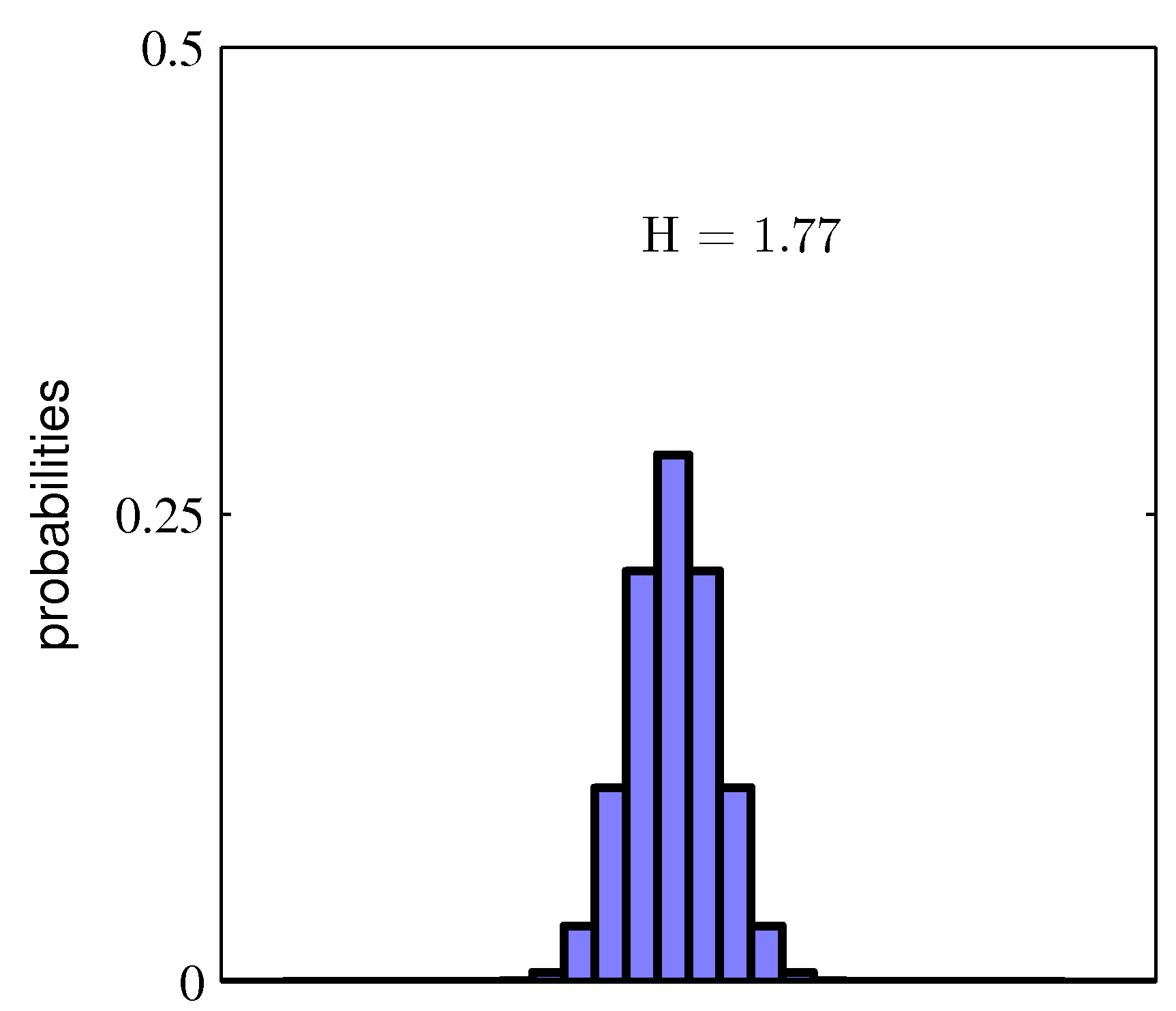
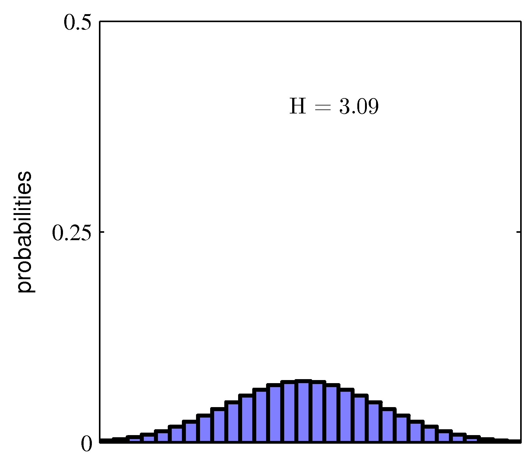
The entropy of a discrete distribution \(p\) measures its average information content:

\[\mathbb{H}[X] = -\sum_x p(x) \log p(x). \tag{1.13}\]

(Use natural log for nats; base-2 log for bits.) Properties:

• \(\mathbb{H}[X] \geq 0\), with equality iff \(p\) is concentrated on one value.
• For a discrete variable with \(K\) outcomes, \(\mathbb{H}[X] \leq \log K\), attained by the uniform distribution.

For a continuous variable, replace the sum with an integral; this is differential entropy (and can be negative).

Kullback–Leibler divergence

Given two distributions \(p\) and \(q\) over the same variable, the KL divergence

\[\mathrm{KL}(p \| q) = -\int p(\mathbf{x}) \log \frac{q(\mathbf{x})}{p(\mathbf{x})}\, \mathrm{d}\mathbf{x} = \int p(\mathbf{x}) \log \frac{p(\mathbf{x})}{q(\mathbf{x})}\, \mathrm{d}\mathbf{x} \tag{1.14}\]

measures how far \(q\) is from \(p\), in the sense of “extra information needed to encode \(p\)-distributed data using a code optimized for \(q\).”

Key properties:

• \(\mathrm{KL}(p \| q) \geq 0\), with equality iff \(p = q\) almost everywhere. (Proof: Jensen’s inequality applied to the convex function \(-\log\).)
• Asymmetric: \(\mathrm{KL}(p \| q) \neq \mathrm{KL}(q \| p)\) in general. This matters when fitting an approximating distribution — see chapter 10.

Mutual information

For two variables \(X\) and \(Y\), the mutual information quantifies how much knowing one tells you about the other:

\[\mathrm{I}[X, Y] = \mathrm{KL}\bigl(p(X, Y) \,\|\, p(X)\, p(Y)\bigr). \tag{1.15}\]

It is zero iff \(X\) and \(Y\) are independent, and positive otherwise. Equivalently, \(\mathrm{I}[X, Y] = \mathbb{H}[X] - \mathbb{H}[X \mid Y] = \mathbb{H}[Y] - \mathbb{H}[Y \mid X]\) — the reduction in uncertainty about \(X\) once you observe \(Y\).

Why this matters for ML

• Maximum likelihood = minimum KL. Given true distribution \(p^{\star}\) and model \(p_\theta\), drawing i.i.d. samples and maximizing \(\sum \log p_\theta(\mathbf{x}_n)\) is, in expectation, equivalent to minimizing \(\mathrm{KL}(p^{\star} \| p_\theta)\).
• Cross-entropy loss. The cross-entropy \(-\sum p^{\star}(x) \log p_\theta(x)\) used to train classifiers is just the entropy of \(p^{\star}\) plus \(\mathrm{KL}(p^{\star} \| p_\theta)\) — minimizing it minimizes KL.
• Variational inference. When the posterior \(p(\mathbf{w} \mid \mathcal{D})\) is intractable, fit an approximating \(q\) by minimizing \(\mathrm{KL}(q \| p)\) — chapter 10.

---

Takeaways

• Linear-in-parameters models can be fit in closed form by solving a linear system — no iteration needed. The polynomial example is the prototype.
• Overfitting is real: enough capacity will memorize training data while failing on new inputs. Defenses: more data, regularization, model selection.
• Probability is the right language for ML. The sum, product, and Bayes’ rules let you reason about parameters as random variables and turn any model into a posterior over \(\mathbf{w}\).
• Decision theory turns posteriors into actions: pick the class minimizing expected loss; for squared regression loss the optimum is the conditional mean.
• Information theory unifies several training objectives. Entropy, KL, and mutual information will reappear in nearly every later chapter.

Forward to Ch 2 — Probability Distributions, where we build the standard distributional toolbox (Bernoulli, Gaussian, exponential family) and their conjugate priors.

---

Figures from Bishop, Pattern Recognition and Machine Learning (Springer, 2006), © Springer / C. M. Bishop. Reproduced for educational use.