Ch 6 — Kernel Methods
Dual representations, kernel functions, the kernel trick, Gaussian processes.
A useful mental shift: many linear-model algorithms can be rewritten so they depend on inputs only through pairwise inner products \(\mathbf{x}_n^{\top}\mathbf{x}_m\). That observation lets us replace the inner product with a more general kernel \(k(\mathbf{x}_n, \mathbf{x}_m)\) — implicitly working in a high (sometimes infinite) dimensional feature space without ever computing the features. This is the kernel trick, and it powers SVMs, RVMs, and Gaussian processes.
Prerequisites
- Linear regression (Ch 3) — kernel ridge regression is the dual of standard ridge.
- Multivariate Gaussians (Ch 2) — Gaussian processes are infinite-dimensional Gaussians.
- Linear algebra — eigendecomposition, positive-definite matrices.
6.1 Dual Representations
Take ridge regression with a feature map \(\boldsymbol{\phi}\). The regularized objective is
\[J(\mathbf{w}) = \frac{1}{2} \sum_{n=1}^{N} (\mathbf{w}^{\top}\boldsymbol{\phi}_n - t_n)^{2} + \frac{\lambda}{2}\\|\mathbf{w}\\|^{2}.\]Setting \(\nabla_{\mathbf{w}} J = 0\) and rearranging shows \(\mathbf{w}\) is a linear combination of the training features:
\[\mathbf{w} = \sum_{n=1}^{N} a_n\, \boldsymbol{\phi}_n, \qquad a_n = \frac{1}{\lambda}(t_n - \mathbf{w}^{\top}\boldsymbol{\phi}_n).\]Substituting back yields a problem entirely in terms of the Gram matrix \(K_{nm} = \boldsymbol{\phi}_n^{\top}\boldsymbol{\phi}_m = k(\mathbf{x}_n, \mathbf{x}_m)\):
\[\mathbf{a} = (\mathbf{K} + \lambda \mathbf{I}_N)^{-1}\mathbf{t}, \qquad y(\mathbf{x}) = \mathbf{k}(\mathbf{x})^{\top}(\mathbf{K} + \lambda \mathbf{I}_N)^{-1}\mathbf{t}, \tag{6.1}\]where \(\mathbf{k}(\mathbf{x})\) has entries \(k_n(\mathbf{x}) = k(\mathbf{x}, \mathbf{x}_n)\). The features \(\boldsymbol{\phi}\) never appear explicitly — only through the kernel.
The trade-off: solving in feature space costs \(O(M^3)\) (with \(M\) features); the dual costs \(O(N^3)\) (with \(N\) data points). Use the dual when \(N \ll M\) (or \(M = \infty\)).
6.2 Constructing Kernels
A function \(k(\mathbf{x}, \mathbf{x}’)\) is a valid kernel iff the Gram matrix \(\mathbf{K}\) is positive semi-definite for every choice of training points (Mercer’s theorem). Common kernels:
| Name | \(k(\mathbf{x}, \mathbf{x}’)\) | Notes |
|---|---|---|
| Linear | \(\mathbf{x}^{\top}\mathbf{x}’\) | Plain inner product. |
| Polynomial | \((\mathbf{x}^{\top}\mathbf{x}’ + c)^{M}\) | Implicit polynomial features up to order \(M\). |
| Gaussian (RBF) | \(\exp(-\|\mathbf{x}-\mathbf{x}’\|^2 / (2\sigma^2))\) | Infinite-dimensional feature space. The default. |
| Matérn-\(\nu\) | parametric family with controlled smoothness | Used in geostatistics and spatial models. |
| Periodic | \(\exp(-2\sin^2(\pi(x-x’)/p)/\sigma^2)\) | Encodes a known period. |
| String / graph | various | Operate on non-vector inputs (text, molecules). |
Useful closure properties: if \(k_1, k_2\) are kernels, so are \(\alpha k_1\) (\(\alpha > 0\)), \(k_1 + k_2\), \(k_1 k_2\), \(\exp(k_1)\), \(f(\mathbf{x}) k_1 f(\mathbf{x}’)\), and \(k_1(g(\mathbf{x}), g(\mathbf{x}’))\). Kernel engineering is mostly composing simple primitives this way.
6.3 Radial Basis Function Networks
Earlier (Ch 3) we used Gaussian RBFs as fixed basis functions centered at chosen locations. The kernel-method perspective makes this less arbitrary: place a basis function on every training point — i.e., the feature map is \(\boldsymbol{\phi}(\mathbf{x}) = (k(\mathbf{x}, \mathbf{x}_1), \ldots, k(\mathbf{x}, \mathbf{x}_N))^{\top}\). This is precisely what equation (6.1) does, with \(N\) basis functions automatically chosen to cover the data.
6.4 Gaussian Processes
A Gaussian process is a distribution over functions \(y(\mathbf{x})\) such that any finite collection of values \(\lbrace y(\mathbf{x}_1), \ldots, y(\mathbf{x}_N)\rbrace\) is jointly Gaussian. It’s specified by:
- A mean function \(m(\mathbf{x})\) — usually taken to be zero.
- A covariance function \(k(\mathbf{x}, \mathbf{x}’)\) — i.e., a kernel.
The kernel encodes prior beliefs about the function: smoothness (RBF), periodicity (periodic), trends (linear).
GP regression
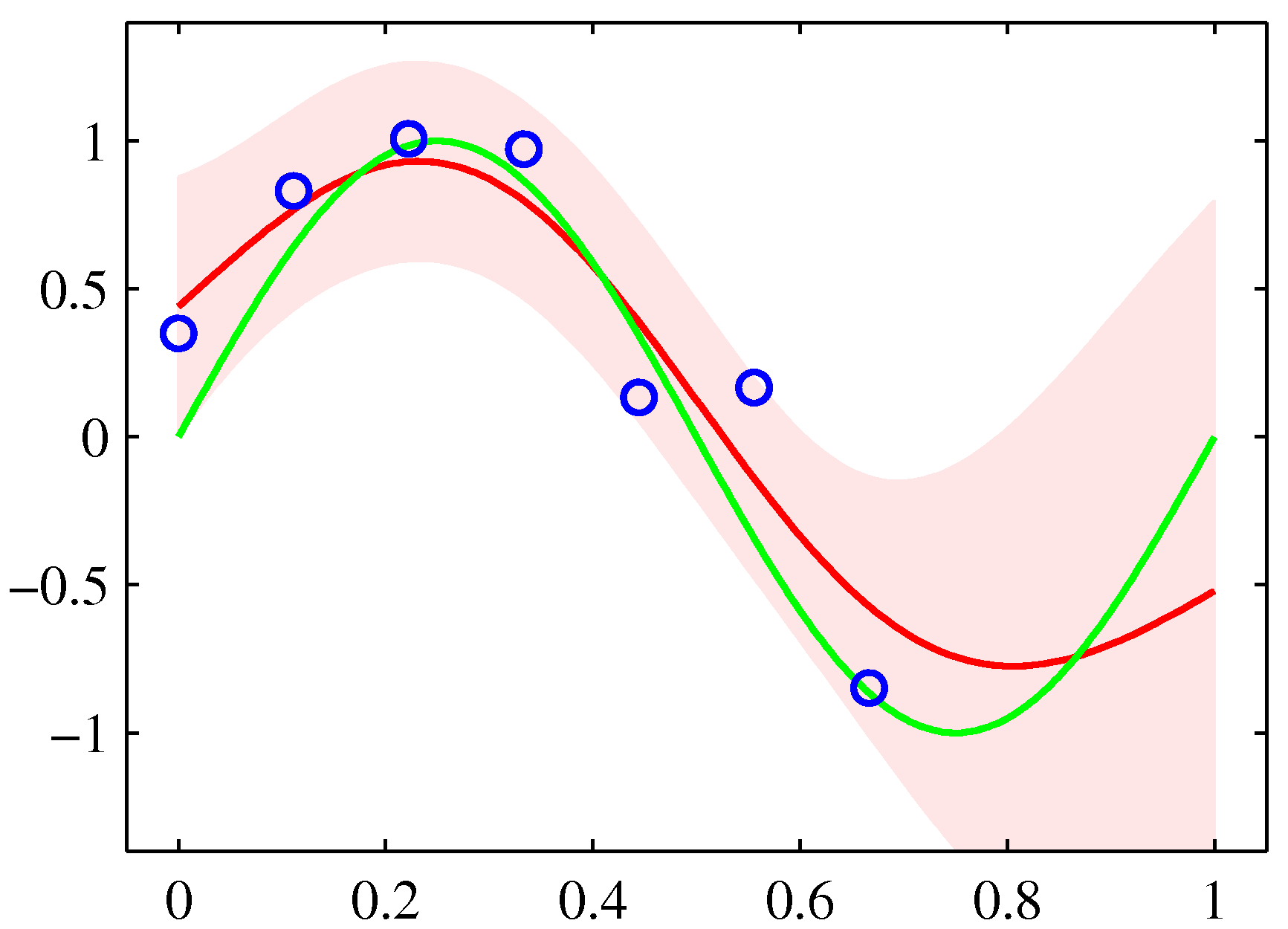
Training data \(\lbrace (\mathbf{x}_n, t_n)\rbrace\) with Gaussian noise \(t = y(\mathbf{x}) + \epsilon\), \(\epsilon \sim \mathcal{N}(0, \beta^{-1})\). For a new \(\mathbf{x}_*\), the predictive distribution is Gaussian:
\[\begin{aligned} m(\mathbf{x}_*) &= \mathbf{k}_*^{\top}\, \mathbf{C}_N^{-1}\, \mathbf{t}, \\ \sigma^{2}(\mathbf{x}_*) &= c - \mathbf{k}_*^{\top}\, \mathbf{C}_N^{-1}\, \mathbf{k}_*, \end{aligned} \tag{6.2}\]where \(\mathbf{C}_N = \mathbf{K} + \beta^{-1}\mathbf{I}\) and \(\mathbf{k}_* = (k(\mathbf{x}_*, \mathbf{x}_1), \ldots, k(\mathbf{x}_*, \mathbf{x}_N))^{\top}\). The mean is the same as the kernel-ridge prediction; the variance grows away from training points, just like Bayesian linear regression’s predictive variance.
GP classification
Replace the Gaussian likelihood with a sigmoid: \(p(t = 1 \mid y) = \sigma(y)\). The posterior over \(y\) is no longer Gaussian, and the predictive distribution requires approximation (Laplace, EP, variational). Same kernel-trick story; harder math.
Hyperparameter selection
Maximize the log marginal likelihood
\[\ln p(\mathbf{t} \mid \boldsymbol{\theta}) = -\tfrac{1}{2} \mathbf{t}^{\top}\mathbf{C}_N^{-1}\mathbf{t} - \tfrac{1}{2}\ln |\mathbf{C}_N| - \tfrac{N}{2}\ln(2\pi)\]with respect to the kernel hyperparameters \(\boldsymbol{\theta}\) (length-scales, noise level, signal variance). The first term rewards data fit; the second penalizes complexity. Same Bayesian-Occam logic as the evidence framework of Ch 3.
6.5 Practicalities
- Cost. GP regression is \(O(N^3)\) in training, \(O(N^2)\) in prediction, due to the matrix inverse. Approximations (sparse GPs, inducing points) reduce to \(O(NM^2)\) for \(M \ll N\).
- Scalability. For \(N \gtrsim 10^4\), exact GPs become impractical. Modern alternatives: variational sparse GPs, deep kernel learning (combining a neural feature extractor with a GP head), or simply a Bayesian neural network.
- When to choose GPs over NNs. Small data, well-calibrated uncertainty needed, smooth / structured response surfaces, non-vector inputs with a hand-engineered kernel.
Takeaways
- The kernel trick lets you work in implicit (high or infinite) feature spaces by using only \(k(\mathbf{x}, \mathbf{x}’)\). The dual cost is \(O(N^3)\) instead of \(O(M^3)\).
- Valid kernels = positive-definite Gram matrices. Common families compose freely (sum, product, exponential).
- Gaussian processes are non-parametric Bayesian models: priors over functions, closed-form posteriors for regression, principled hyperparameter selection via marginal likelihood.
- GPs scale poorly past ~10 k points; approximations and modern alternatives bridge to deep learning territory.
Forward to Ch 7 — Sparse Kernel Machines (SVM, RVM).
Figures from Bishop, Pattern Recognition and Machine Learning (Springer, 2006), © Springer / C. M. Bishop. Reproduced for educational use.