PyTorch Transfer Learning
Reusing pretrained models — freezing feature extractors, replacing classifier heads, and fine-tuning on a small custom dataset.
In 06 PyTorch Going Modular we wrapped the training pipeline into reusable scripts. The model itself — TinyVGG — only got us to about 40 % test accuracy on pizza/steak/sushi, because there simply isn’t enough custom data to learn good visual features from scratch.
The fix is transfer learning: take a model that already learned good visual features on a huge dataset (typically ImageNet, ~1.3M images, 1000 classes) and reuse those features for our 225-image, 3-class problem. Same dataset, same training script, just a different model class — and accuracy jumps to ~85 %.
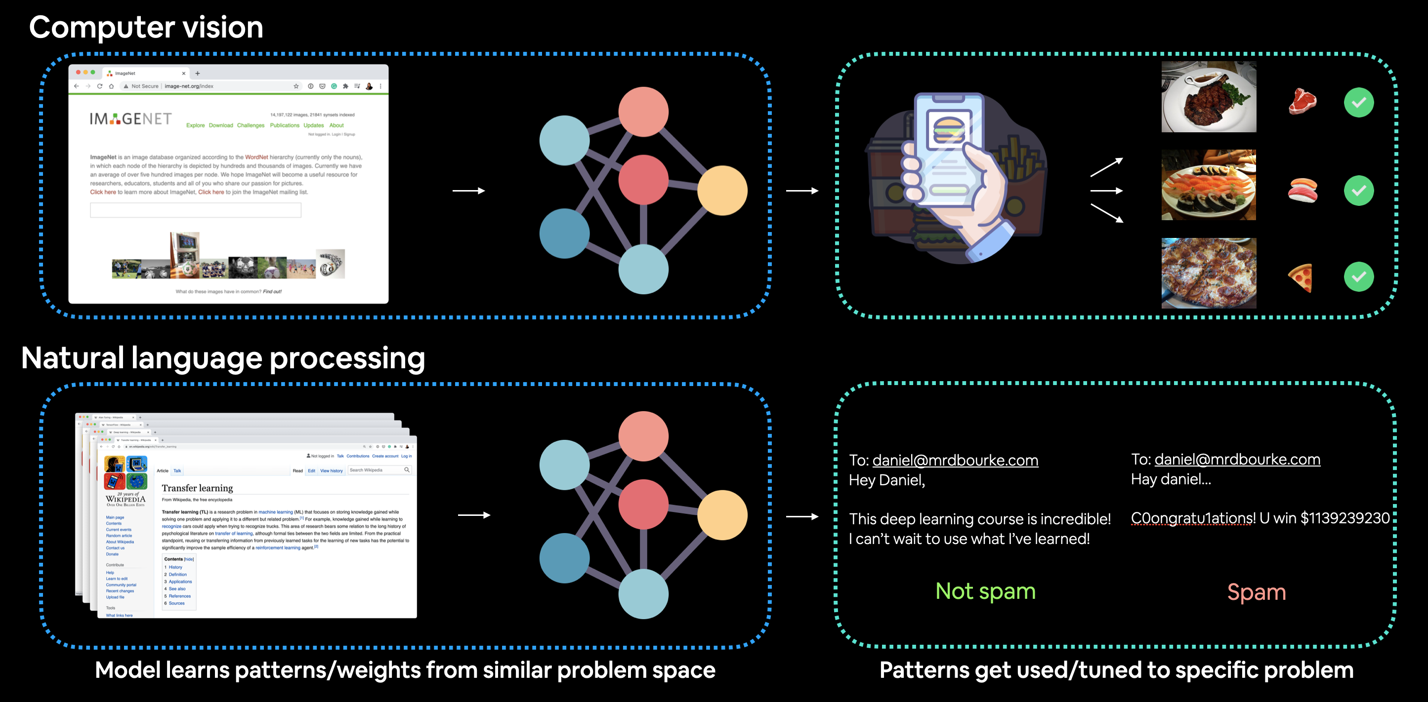
What is transfer learning?
Transfer learning is the practice of taking a model that was trained on task A and adapting it for task B, on the assumption that A and B share underlying structure. For images this assumption holds extraordinarily well: edges, corners, textures, and parts are useful whether you’re classifying ImageNet’s 1000 categories or three kinds of food.
Concretely, every modern image-classification network has the shape:
input → feature extractor → classifier head → output logits
The feature extractor (early conv layers) learns generic visual primitives. The classifier head (the final one or two Linear layers) maps those features to the specific output classes. To transfer, we keep the feature extractor’s weights frozen and replace the classifier head with one shaped for our classes.
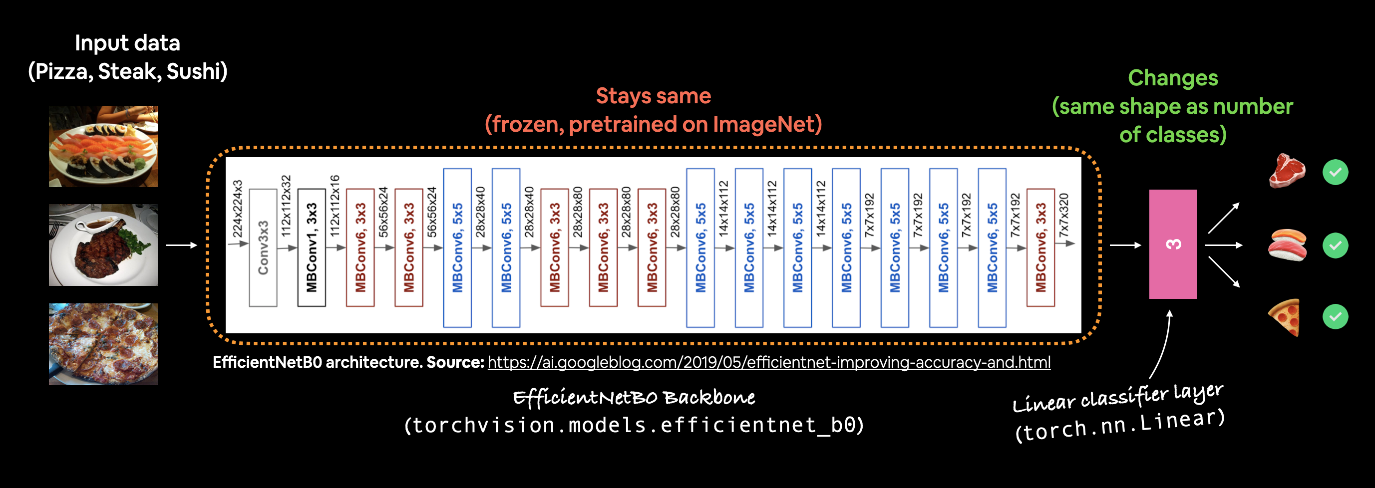
Two practical wins:
- Strong baseline with little data. A frozen ImageNet feature extractor already produces excellent features; the classifier head only has to learn a small linear mapping.
- Fast to train. With the base layers frozen, only the head’s parameters get updated. Backprop touches a few thousand parameters instead of a few million.
Where to find pretrained models
| Source | What’s there |
|---|---|
torchvision.models |
Battle-tested vision models — ResNet, VGG, EfficientNet, ViT, ConvNeXt — all with ImageNet weights. The default for most projects. |
timm (rwightman/pytorch-image-models) |
The largest collection of state-of-the-art vision architectures in PyTorch, often with weights from multiple training recipes. |
| HuggingFace Hub (huggingface.co/models) | Thousands of models across vision, text, audio. Especially strong for transformer architectures. |
| Papers With Code (paperswithcode.com) | Tracks SOTA per benchmark, links to public implementations and weights. |

For this lesson we’ll use torchvision.models.efficientnet_b0 — small enough to train on a laptop, accurate enough that you’ll see a clear improvement over TinyVGG.
What we’re going to do
- Reuse
data_setup,engine,utilsfrom the previous lesson. - Build DataLoaders, but use the correct preprocessing for our pretrained model.
- Download
efficientnet_b0with ImageNet weights. - Freeze all the convolutional feature layers.
- Replace the final classifier with a fresh head whose output size = 3.
- Train for a handful of epochs.
- Compare with TinyVGG and predict on a few custom images.
1. Data: matching the pretrained model’s preprocessing
This step matters more than people expect. A pretrained model expects its input to look exactly like the data it was trained on. Different mean/std, different resize, even a different interpolation can quietly degrade accuracy.
The manual way (works on any torchvision version)
ImageNet’s per-channel statistics are the canonical normalization values:
from torchvision import transforms

manual_transform = transforms.Compose([
    transforms.Resize((224, 224)),
    transforms.ToTensor(),                                  # [0, 1]
    transforms.Normalize(mean=[0.485, 0.456, 0.406],        # ImageNet mean
                         std =[0.229, 0.224, 0.225]),       # ImageNet std
])
Then build DataLoaders the usual way:
from going_modular import data_setup
train_dl, test_dl, class_names = data_setup.create_dataloaders(
    train_dir="data/pizza_steak_sushi/train",
    test_dir ="data/pizza_steak_sushi/test",
    transform=manual_transform,
    batch_size=32,
)
The automatic way (torchvision ≥ 0.13)
Recent torchvision ships the exact preprocessing pipeline alongside each set of pretrained weights. No more guessing about mean/std:
import torchvision

weights = torchvision.models.EfficientNet_B0_Weights.DEFAULT
auto_transform = weights.transforms()

train_dl, test_dl, class_names = data_setup.create_dataloaders(
    train_dir="data/pizza_steak_sushi/train",
    test_dir ="data/pizza_steak_sushi/test",
    transform=auto_transform,
    batch_size=32,
)
Whenever it’s available, prefer the automatic transform — it’s guaranteed to match how the weights were trained.
2. Loading a pretrained model
The modern API takes a weights= argument instead of the deprecated pretrained=True:
weights = torchvision.models.EfficientNet_B0_Weights.DEFAULT
model = torchvision.models.efficientnet_b0(weights=weights).to(device)
weights.DEFAULT always points to the most accurate set of ImageNet weights torchvision ships for that architecture. If you want a specific recipe (e.g. IMAGENET1K_V1 vs IMAGENET1K_V2), pass it explicitly.
Print the model’s top-level structure:
print(model)
You’ll see three sections:
features— a stack ofMBConvblocks (the convolutional feature extractor).avgpool— adaptive average pooling that produces a 1280-dim feature vector regardless of input size.classifier—Dropout(0.2) → Linear(1280 → 1000). The 1000 output classes are ImageNet’s, not ours.
3. Freezing the feature extractor
Freezing means don’t compute gradients for, and don’t update, these parameters. We achieve it by setting requires_grad = False:
for param in model.features.parameters():
    param.requires_grad = False
After this loop, only the parameters in model.classifier (and any unfrozen layers) will receive gradient updates. PyTorch’s optimizer simply skips parameters whose requires_grad is False.
4. Replacing the classifier head
The default head outputs 1000 logits. Our problem has 3 classes (pizza, steak, sushi), so we need a new head with output size 3.
import torch
from torch import nn

torch.manual_seed(42)  # reproducibility

model.classifier = nn.Sequential(
    nn.Dropout(p=0.2, inplace=True),
    nn.Linear(in_features=1280, out_features=len(class_names)),  # 3
).to(device)
A few notes:
- Keep the
Dropout(p=0.2)— it’s part of how this model was originally trained. 1280is fixed by EfficientNet-B0’s feature dimension. Different architectures (ResNet-50: 2048; ViT-B/16: 768) have different numbers — always read it off the model.- The new layer is initialized randomly. After freezing, this is the only set of parameters being trained.
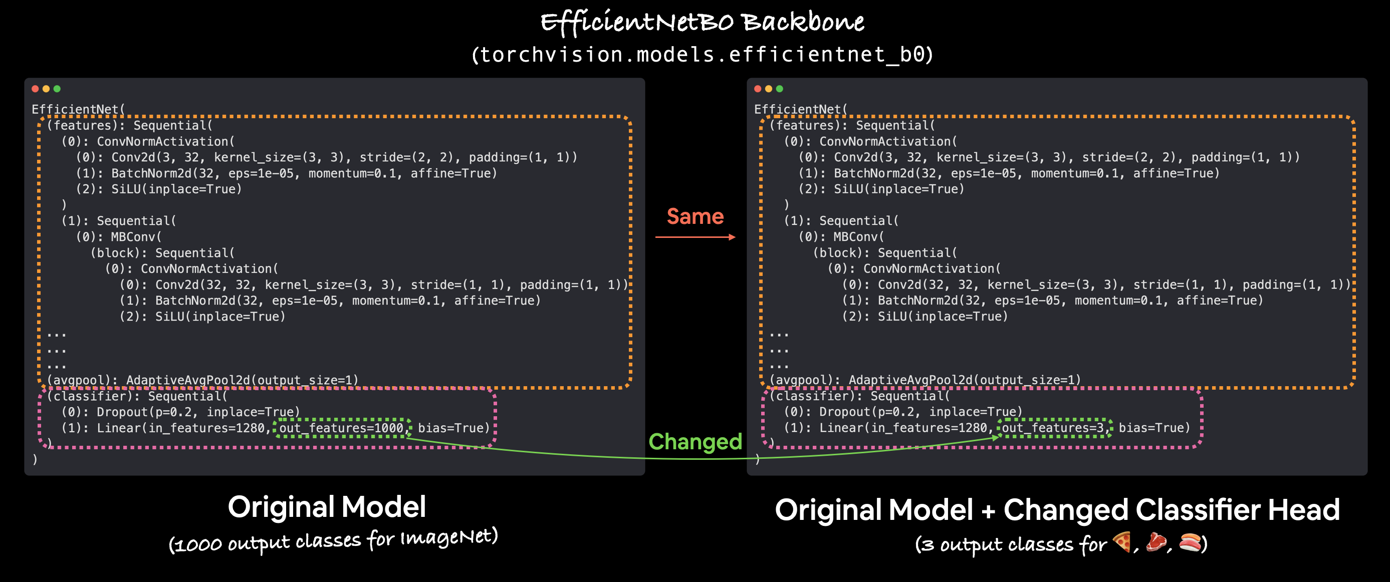
Linear(1280, 3) that maps to our pizza / steak / sushi classes.
A quick sanity check:
from torchinfo import summary
summary(model, input_size=(1, 3, 224, 224))
You’ll see tens of millions of parameters in features (frozen, marked Trainable: False) and a few thousand in classifier (trainable). For EfficientNet-B0 with three output classes the trainable count is 3,843. That’s why training is fast.
5. Training
We can reuse engine.train from the previous chapter unchanged:
from going_modular import engine

loss_fn   = nn.CrossEntropyLoss()
optimizer = torch.optim.Adam(model.parameters(), lr=1e-3)
# Adam ignores parameters with requires_grad=False, so freezing is respected.

results = engine.train(
    model=model,
    train_dataloader=train_dl,
    test_dataloader=test_dl,
    optimizer=optimizer,
    loss_fn=loss_fn,
    epochs=5,
    device=device,
)
After 5 epochs (~10 seconds on a free Colab GPU) you should see test accuracy north of 80 %. Compare that to TinyVGG’s ~40 % from the previous lesson — same data, same training loop, much better features.
6. Looking at the loss curves
Plotting results makes the picture obvious:
import matplotlib.pyplot as plt

epochs = range(1, len(results["train_loss"]) + 1)

fig, ax = plt.subplots(1, 2, figsize=(10, 4))
ax[0].plot(epochs, results["train_loss"], label="train")
ax[0].plot(epochs, results["test_loss"],  label="test")
ax[0].set_title("Loss");      ax[0].legend()
ax[1].plot(epochs, results["train_acc"], label="train")
ax[1].plot(epochs, results["test_acc"],  label="test")
ax[1].set_title("Accuracy");  ax[1].legend()
plt.show()
What to look for:
- Train and test loss both decreasing → learning normally.
- Train loss « test loss for many epochs → starting to overfit. Add data augmentation, increase dropout, or freeze more / fewer layers.
- Test accuracy plateaus quickly → you may have hit the ceiling for a frozen feature extractor; the next step is fine-tuning (unfreezing the top few feature blocks and training with a small learning rate).
7. Predicting on custom images
Once you’re happy with the trained model, run it on images outside the dataset:
from PIL import Image
import torch

def predict(model, image_path, transform, class_names, device):
    img = Image.open(image_path).convert("RGB")
    x = transform(img).unsqueeze(0).to(device)              # (1, 3, 224, 224)
    model.eval()
    with torch.inference_mode():
        logits = model(x)
        probs  = torch.softmax(logits, dim=1)
        pred   = class_names[probs.argmax(dim=1).item()]
    return pred, probs.max().item()

label, conf = predict(model, "my_pizza.jpg",
                      transform=auto_transform,
                      class_names=class_names,
                      device=device)
print(f"prediction: {label}  ({conf*100:.1f}% confidence)")
Two things easy to forget:
- Use the same transform you trained with. If you used
auto_transformfor training, use it here too. Mismatched preprocessing is the single most common cause of “the model is great in the notebook but garbage in production.” - Open the image as RGB. Some files are RGBA or grayscale;
.convert("RGB")makes the channel count consistent.
What to try next: fine-tuning
Freezing the feature extractor is “transfer learning, easy mode.” The next step is fine-tuning: unfreeze the last few feature blocks and re-train them with a much smaller learning rate (typically 10–100× smaller than the head’s lr). This nudges the late-stage features to adapt to your domain without erasing what they learned on ImageNet.
# Unfreeze the last block
for param in model.features[-1].parameters():
    param.requires_grad = True

# Use a smaller lr for the unfrozen base
optimizer = torch.optim.Adam([
    {"params": model.classifier.parameters(),    "lr": 1e-3},
    {"params": model.features[-1].parameters(),  "lr": 1e-5},
])
For 225 images this isn’t usually worth it — but on a few thousand domain-specific images it often pushes accuracy a few more points.
Takeaways
- Always ask “is there a pretrained model for this?” before designing an architecture from scratch.
- Match the preprocessing. Use
weights.transforms()whenever you can; otherwise reproduce the original mean/std/resize exactly. - Freeze first, fine-tune later. Replace the head and train it alone before unfreezing any feature layers.
- Read the output dimension off the model. EfficientNet-B0’s 1280, ResNet-50’s 2048, ViT-B/16’s 768 — they aren’t interchangeable.
- Same engine, better model. The training loop you wrote in chapter 06 didn’t change at all; the gain came entirely from a better starting point.